This chapter explains how to find solutions to several problems in Operations Research. More specifically, they are problems in Linear Programming (LP) and Integer Programming (IP) where the solution is found as the optimal value of an objective function subject to the existence of various constraints, all of which are expressed as linear functions. The difference between LP and IP is the possible values for the decision variables under consideration.
To benefit the most from this chapter, you ought to be familiar with basic manipulation of vectors and matrices, as seen in Chapter 21 and be ready to install an additional package using the methods outlined in Chapter 16. You will need to install the lpSolve package and make sure it is ready for use by calling the require() command as seen in the examples in this chapter. Note that this need only be done once, but the command is repeated as a reminder.
Note that all examples are intentionally made reproducible through use of random number generation. You will need to make sure you reset the random number generator’s seed value using the set.seed() commands that appear in the examples.
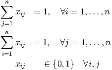
The assignment problem assigns n tasks to n people. The objective function is often described in tabular or matrix form as a set of costs to be minimised. The constraints are that all tasks must be assigned and no person can complete more than one task. “Dummy" tasks or people are added to the matrix if the number of tasks is not equal to the number of people.
The mathematical programming representation for the assignment problem has the objective function:
 | (22.1) |
subject to the constraints:

Note that the print out of the solution didn’t actually tell us which task was to be completed by which person so we needed to look for the matrix of the final values for the decision variables. There are plenty of additional items stored as part of the solution, many of which you may never need. It is assumed that if your needs run to the advanced ideas using these items that you will now know where to find the necessary information to solve your own problems.
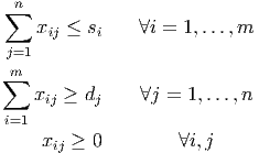
The transportation problem aims to satisfy the demands of a set of customers by optimising the selection of the supplier who will meet each customer’s demands. The mathematical program for this problem has a cost matrix and upper bounds on supply and lower bounds on demands. The optimisation is a minimisation exercise so the demand is kept as low as is required so the lower bounds are (in essence) equality constraints as a consequence.
The objective function is:
 | (22.2) |
and the constraints are:
