Chapter4 Poisson Regression: Models for Count Data
Chapter Aim: To introduce a model which permits the response variable to be a count, with a mean value equal to (almost) any function of a linear combination of predictor variables.
4.1 The Generalised Linear Model for a Poisson Response
The generalised linear model has three components
\(\boldsymbol{\beta}^{\mathrm{T}}\boldsymbol{x}\) a function of the explanatory variables linear in the parameters. The explanatory variables still must be linear in the parameters.
\(Y_i\) are independently observed response variables sharing the same family of distributions. The response need not have a normal distribution.
\(g(\mu_i) = \boldsymbol{\beta}^{\mathrm{T}}\boldsymbol{x}\), a monotonic link function g. \(\mathrm{E}(Y_i) = \mu_i\) need not be a linear function of the explanatory variable(s).
These three components are also the core assumptions of a generalised linear model. The important feature of the model is that the variability of the response can be modeled independently of its mean. Remember that for a transformation to both give Y a constant variance and make it a linear function of \(\boldsymbol{x}\) requires a fortunate coincidence. With a generalised linear model no such coincidence is required.
Sometimes it is useful to label \(\boldsymbol{\beta}^{\mathrm{T}}\boldsymbol{x}_i\) as \(\eta_i\), the linear predictor. Then g must be monotonic so that \(g(\mu_i) = \boldsymbol{\beta}^{\mathrm{T}}\boldsymbol{x}_i = \eta_i\) can be reversed:
\[\begin{align} \mu_i & = g^{-1}(\boldsymbol{\beta}^{\mathrm{T}}\boldsymbol{x}_i) & = g^{-1}(\eta_i) \tag{4.1} \\ \eta_i & = \boldsymbol{\beta}^{\mathrm{T}}\boldsymbol{x}_i \qquad & = g(\mu_i ) \tag{4.2} \end{align}\]
There are technical limitations on the distribution of \(Y_i\) which we will discuss later. Often the distribution will have one parameter, like p with the binomial or \(\lambda\) with the Poisson, which will determine the mean. For example \(\mu=np\) for the binomial and \(\mu=\lambda\) for the Poisson. The variance will also depend on this parameter. For the binomial \(\sigma^2 = np(1-p)\) and for the Poisson \(\sigma^2 = \lambda\). The ‘normal’ distribution is abnormal in having a variance which is independent of its mean. Usually even distributions which have a second parameter changing their scale will still have a variance depending on their mean. For example the variance of the gamma distribution is \(\phi\mu^2\), where \(\phi\) is a scale parameter.
All the above distributions have a boundary at zero. You have probably already noticed that confidence intervals for p can sometimes have negative lower limits. These arise from the assumption that the statistic \(\hat{p}\) has a normal distribution and therefore constant variance. We will see in Chapter 5 that a generalised linear model uses the correct binomial variance. This is much smaller when p is close to zero, shortening the confidence interval and keeping the lower limit non-negative.
Boundary effects are an important, but extreme example of where the ordinary linear model might break down. In most real data sets the variance depends to some extent on the mean, perhaps not enough to seriously affect the estimates from a linear model, but enough to make it well worthwhile having another tool available. The generalised linear model is that tool.
4.1.1 Example: AIDS deaths in Australia
| Period | 1 | 2 | 3 | 4 | 5 | 6 | 7 | 8 | 9 | 10 | 11 | 12 | 13 | 14 |
| Deaths | 0 | 1 | 2 | 3 | 1 | 4 | 9 | 18 | 23 | 31 | 20 | 25 | 37 | 45 |
The data in Table 4.1 were taken from (Dobson 1990) and show the numbers of deaths from AIDS in Australia per quarter from the first quarter of 1983 to the second quarter of 1986. The data are plotted in Figure 4.1.
For any epidemic the rate of growth in the early stages is proportional to the number of infected people. This leads to an exponential process, so the mean number of deaths at time period t, denoted \(\mu_t\), increases exponentially with time, t. \[\mu_t = e^{\beta t} \qquad \leftrightarrow \qquad \ln ( \mu_t) = \beta t\] Remember that the log function used as the inverse to the exponential function is log to base e, which is why we use \(ln\) rather than \(log_{10}\).
There is a large population of people at risk, and each has a very small probability of dying in any three-month period. In practice, each individual would have a different probability, but as a first approximation assuming that the probability is constant over all the “at risk" population, and that therefore the distribution is Poisson, should give a reasonable approximate model.
A generalised linear model is the result:
The linear function \(\boldsymbol{\beta}^{\mathrm{T}}\boldsymbol{x}_i\) is just \(\beta t = \eta_t\). Here the vectors \(\boldsymbol{\beta}\) and \(\boldsymbol{x}\) have just one element.
\(Y_t\) has a Poisson distribution with mean \(\mu_t\)
\(\ln(\mu_t) = \beta t\); the natural logarithm function is the link
The plot shows that the variability increases with the mean, as expected with a Poisson distribution. The theory of Chapter 2 said that a square root transformation would even it out, but a log transformation is needed to straighten the curve. A GLM (Generalised Linear Model) models both the Poisson and the curve.
    data(Aids, package="ELMER")
    Aids.glm<-glm(Deaths~-1+Period,family=poisson(link="log"),data=Aids)
    plot(Aids$Period,Aids$Deaths,xlab="Period",ylab="Deaths",cex.lab=1.5)
    lines(exp(Aids.glm$coef[1]*Aids$Period))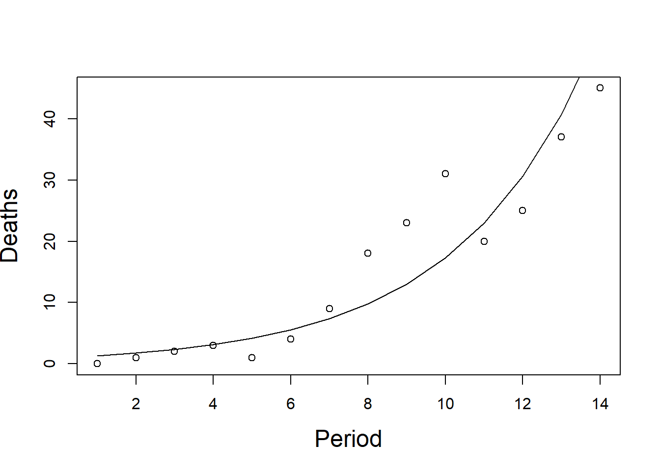
Figure 4.1: Numbers of deaths from AIDS in Australia per quarter from 1983 to 1986. Line shows \(e^{0.285t}\), the generalised linear model with Poisson errors.
4.2 Computing discussion
Any program which fits generalised linear models will give the estimates for this model almost as easily as an ordinary linear model. The only information required is the link function (g) and the distribution of Y. The output is in the same form as you are given from an ordinary linear regression.
The method used is based on the iterative process described in Chapter 3. The next section extends the iterative process in an empirical way, then the following section shows that this process is equivalent to maximum likelihood.
4.3 Empirical argument
Because \(Y_t\) has a Poisson distribution, \(var(Y_t) = \mu_t\). Can we modify the method of Chapter 3 to estimate \(\beta\)? The difficulty is that we know the variance of \(Y_t\), but the linear model is fitted to \(\ln(Y_t)\). The weight should be \(1/var(ln(\mu_t))\), but this cannot be written as a simple function.
The solution is to use the same method as that used to derive Equation (2.15) \[FindFTransformation\] to linearise the transformation.
\[\begin{align} \ln(y_t) & = \ln(\mu_t) + \frac{d\left[\ln(\mu_t)\right]}{d\mu_t} (y_t-\mu_t) + \textrm{small terms} \notag \\ & \approx \ln(\mu_t) + \frac{1}{\mu_t}(y_t-\mu_t) \notag \\ & \approx \eta + \frac{y_t -\mu_t}{\mu_t} \tag{4.3}\\ \end{align}\]
This approximate, linearised form of the equation is used as the response variable. From it we can calculate an approximate variance: \[var\left(\eta + \frac{Y_t - \mu_t}{\mu_t}\right) = \frac{1}{\mu_t^2}var(Y_t) = \frac{1}{\mu_t}\] So if \(\hat{\mu}_{(0)}\) is a first approximation, which can simply be the data itself with a small constant added to avoid taking logs of zero, \[\begin{equation} \hat{\eta}_{(0)} = \ln(\hat{\mu}_{(0)}) \tag{4.4} \end{equation}\]
Then \(\hat{\beta}_{(1)}\) is estimated by fitting
\[\begin{equation} \hat{\eta}_{(0)t}+\frac{y_t - \hat{\mu}_{(0)t}}{\hat{\mu}_{(0)t}} \tag{4.5} \end{equation}\]
to t using \(\hat{\mu}_{(0)t}\) as weights, thus giving \(\hat{\beta}_{(1)}\) which can then be used to calculate \(\mu_{(1)}\) for a further iteration.
This process will work so long as
the link function is 1-1 to ensure that it can be inverted and its derivative exists.
the variance of Y is a function of \(\mu\) , and perhaps a constant
Note that the precise distribution of Y is not needed, just its variance as a function of its mean.
Finally then, the above describes a sensible looking procedure to use with any 1-1 link function and any data where the variance depends on the mean. Let’s now see the theory applied to some data.
Table 4.2 shows the R code and results of applying this procedure to the AIDS data. Note: The weights used in this model seem to be inconsistent with the approach taken in Chapter 3. It is important to note that in this example, the response variable has been transformed as per Equation (4.4). This has an impact on the weights used in the model fitted, in the code chunk above Table 4.2, which are the reciprocals of the weights used in the previous chapter. Care will need to be taken if you intend to fit a model using an iterative process. Ask yourself if you have used a link function for your response variable; if yes, then the above working is the correct procedure (which we will discuss further in Chapter 6) but if you use an approach based on a known theoretical estimator of the variance and the raw response data, then the approach of Chapter 3 is much simpler to apply.
Although this process should take place inside a computer you will remember from Chapter 3 that iterations do not always converge in a trouble free way. You do need to be aware of what is involved because now and again your friendly computer will tell you that even after lots of iterations it still cannot give you the answers you hoped for.
    Aids$mu.0<-Aids$Deaths+0.1
    loglike.0<-sum(-Aids$mu.0+Aids$Deaths*log(Aids$mu.0)-log(factorial(Aids$Deaths)))
    Aids$z.0<-log(Aids$mu.0)+((Aids$Deaths-Aids$mu.0)/Aids$mu.0)

    Model<-lm(z.0~Period-1,weights=mu.0,data=Aids)
    beta.0<-Model$coeff[1]

    Aids$mu.1<-exp(Model$coeff*Aids$Period)
    loglike.1<-sum(-Aids$mu.1+Aids$Deaths*log(Aids$mu.1)-log(factorial(Aids$Deaths)))
    Aids$z.1<-log(Aids$mu.1)+(Aids$Deaths-Aids$mu.1)/Aids$mu.1

    model2<-lm(z.1~Period-1,weights=mu.1,data=Aids)
    beta.1<-model2$coef[1]

    Aids$mu.2<-exp(model2$coeff*Aids$Period)
    loglike.2<-sum(-Aids$mu.2+Aids$Deaths*log(Aids$mu.2)-log(factorial(Aids$Deaths)))

    #From GLM model
    Aids$mu<-exp(Aids.glm$coef[1]*as.numeric(Aids$Period[1:14]))
    beta.mu<-Aids.glm$coef[1]
loglike.mu<-logLik(Aids.glm)[1]| Period | Deaths | mu.0 | z.0 | mu.1 | z.1 | mu.2 | mu |
|---|---|---|---|---|---|---|---|
| 1 | 0 | 0.1 | -3.3026 | 1.336 | -0.7104 | 1.330 | 1.330 |
| 2 | 1 | 1.1 | 0.0044 | 1.785 | 0.1396 | 1.769 | 1.768 |
| 3 | 2 | 2.1 | 0.6943 | 2.384 | 0.7077 | 2.353 | 2.352 |
| 4 | 3 | 3.1 | 1.0991 | 3.186 | 1.1004 | 3.129 | 3.127 |
| 5 | 1 | 1.1 | 0.0044 | 4.256 | 0.6832 | 4.161 | 4.159 |
| 6 | 4 | 4.1 | 1.3866 | 5.685 | 1.4415 | 5.535 | 5.530 |
| 7 | 9 | 9.1 | 2.1973 | 7.595 | 2.2125 | 7.361 | 7.354 |
| 8 | 18 | 18.1 | 2.8904 | 10.147 | 3.0911 | 9.790 | 9.780 |
| 9 | 23 | 23.1 | 3.1355 | 13.556 | 3.3035 | 13.020 | 13.005 |
| 10 | 31 | 31.1 | 3.4340 | 18.110 | 3.6082 | 17.317 | 17.294 |
| 11 | 20 | 20.1 | 2.9957 | 24.195 | 3.0128 | 23.031 | 22.998 |
| 12 | 25 | 25.1 | 3.2189 | 32.323 | 3.2492 | 30.631 | 30.584 |
| 13 | 37 | 37.1 | 3.6109 | 43.182 | 3.6223 | 40.739 | 40.671 |
| 14 | 45 | 45.1 | 3.8067 | 57.690 | 3.8351 | 54.182 | 54.084 |
| beta.0 | beta.1 | beta.mu |
|---|---|---|
| 0.2896 | 0.2852 | 0.285 |
| loglike.0 | loglike.1 | loglike.2 | loglike.mu |
|---|---|---|---|
| -26.58 | -42.47 | -42.16 | -42.16 |
| where | mu.i: | Predicted values for deaths \(=e^{\beta_{(i)}t}\) at iteration i |
| z.i.: | \(\beta_{(i)}t+(y-\mu_{(i)})/\mu_{(i)}\) | |
| mu: | Predicted values after iterations have converged | |
| beta.i: | Regression of \(z_{(i)}\) on Period using \(\mu_{(i-1)}\) as weight | |
| loglike.i: | Log likelihood or \(\Sigma(-\mu_t + y_t ln(\mu_t )-ln(y_t !))\) |
4.4 Maximum likelihood for Generalised Linear Models
The theory in this section shows that maximum likelihood leads to the same procedure as the empirical method. From the Poisson density function, the contribution to the likelihood from each observation is \[L(\beta;y_t) = e^{-\mu_t}\frac{(\mu_t)^{y_t}}{y_t !}\] where the mean \(\mu_t = e^{\beta t}\). So, since each observation is independent, the likelihood of the sample is \[\prod_t {L(\beta;y_t )} = \prod_t {e^{-\mu_t}\frac{(\mu_t)^{y_t}}{y_t !}}\] Maximum likelihood finds the value of \(\beta\) which maximises this product. As usually is the case, the log of the likelihood is easier to maximise than the likelihood itself, and since log is a monotonic function, the value of \(\beta\) which maximises one also maximises the other. Writing the log of the above likelihood function as \(\ell\) gives
\[\begin{align} \ell(\beta;y) & = \sum_t{ \ln\left(e^{-\mu_t}\frac{(\mu_t)^{y_t}}{y_t !}\right)} \nonumber \\ & = \sum_t{\left( -(\mu_t) + y_t \ln(\mu_t)-\ln(y_t !) \right)} \tag{4.6} \end{align}\]
The usual method of maximising this function is to differentiate \(\ell(\beta;y)\) with respect to \(\beta\) and solve the equation \(\frac{\partial \ell}{\partial \beta} = 0\).
It turns out that the equation to be solved for \(\beta\) is
\[\begin{equation} f(\beta) = \sum_t { t(e^{\beta t} - y_{t})} = 0 \tag{4.7} \end{equation}\]
This does not have an analytical solution, and must be solved numerically. To accomplish this the Newton-Raphson method is used. Please see the appendix to this chapter for the mathematical derivation.
The important implication of this method is that the iteration which generates the new estimate of \(\beta\) is a standard weighted regression process which is built into every statistics regression program.
The calculations are
Find starting estimates, \(\hat{\boldsymbol{\mu}}_{(0)}\), which can be the original data with a small constant added to avoid \(\ln(0)\).
Use this value of \(\hat{\boldsymbol{\mu}}_{(0)}\) to calculate \(z_{t} = \ln(\hat{\mu}_{(0)t}) + \frac{y_{t} - \hat{\mu}_{(0)t}}{\hat{\mu}_{(0)t}}\) for each t.
Calculate a weighted regression of \(z_{t}\) against t using \(\hat{\mu}_{t}\) as the weights.
Use the value of \(\beta\) to calculate \(\hat{\boldsymbol{\mu}}_{(1)}\) and use it to repeat step 2.
Continue until the value of \(\beta\) and \(\ell(\beta;y)\) stabilise.
4.5 Discussion of inference
The generality of these new models is gained at the cost of losing exact inferences. Section 2.3.4 explained the relationship between the distribution of the log-likelihood function and the \(\chi^{2}\) distribution. Figure 2.10 shows that the sharpness of the peak of the log-likelihood function is related to the precision of the estimate. The sharpness of the peak of the curve is measured by the value of the second derivative at its peak. In fact there is a standard result about maximum likelihood estimators of parameters of the exponential family of distributions:
If \(\hat{\beta}\) is the maximum likelihood estimator of \(\beta\),
\(E(\hat{\boldsymbol{\beta}}) \approx \boldsymbol{\beta}\)
\(var(\hat{\boldsymbol{\beta}}) \approx \frac{-\partial^2\left[\ell(\boldsymbol{\beta})\right]}{\partial\boldsymbol{\beta}^2}\) evaluated at \(\hat{\boldsymbol{\beta}}\).
\(\hat{\boldsymbol{\beta}}\) has (approximately) a multivariate normal distribution.
Note that in our example (from Table 4.2)
\[\begin{align} \frac{\partial^2(\ell(\beta))}{\partial \boldsymbol{\beta}^2} & = \sum_{t}{\left(-t^{2} e^{\beta t} \right)} = \sum_{t} {\left(-t^{2}\hat{\mu}_{t}\right)} \notag \\ & = 28813 \notag \\ \textrm{s.e.}(\hat{\beta}) & = (28813)^{-1/2} = 0.00589 \notag \end{align}\]
It is reassuring to note that the formulas do work, but for this course you may assume that the computer will produce the standard errors required. The summary output below shows the results.
Call:
glm(formula = Deaths ~ -1 + Period, family = poisson(link = "log"),
    data = Aids)

Coefficients:
       Estimate Std. Error z value Pr(>|z|)
Period  0.28504    0.00589    48.4   <2e-16 ***
---
Signif. codes:  0 '***' 0.001 '**' 0.01 '*' 0.05 '.' 0.1 ' ' 1

(Dispersion parameter for poisson family taken to be 1)

    Null deviance: 1001.779  on 14  degrees of freedom
Residual deviance:   31.385  on 13  degrees of freedom
AIC: 86.31

Number of Fisher Scoring iterations: 4
This result is an asymptotic result - it becomes more closely true as the sample size increases. Just how large the sample has to be varies from one case to another. For example, if the response has a normal distribution, the result is exact, but if the response has a highly skew distribution a sample of 50+ might still give only rough inferences.
4.6 The Deviance
A crucially important statistic in linear models is the residual sum of squares. The importance of each extra term fitted is assessed by the reduction in residual sum of squares it causes. The comparable quantity in generalised linear models is the deviance. It is derived from the log-likelihood of the model, and for normal linear models it equals the residual sum of squares. The following example shows how close the parallel is between the deviance and the residual sum of squares.
4.6.1 Example: Adding a term to the AIDS model.
The model fitted to the AIDS data was a little unusual in that no constant term was included. Is a constant term needed? In standard linear models questions like this are answered by examining reductions in the residual sum of squares. If the reduction is large relative to the residual from the full model, as measured by an F-test, the extra term(s) are judged significant. The equivalent statistic for GLMs is the deviance, a quantity based on twice the log-likelihood (denoted \(-2 \ell (\beta)\)). In Chapter 2 (Figure 2.10 \[WoolLogLike\] and Equation (2.12) \[CIForLambda\]) changes in \(2\ell(\lambda)\) were used to assess the significance of added parameters. Recall that if the added parameter(s) are zero the change will have (approximately) a \(\chi^{2}\) distribution with degrees of freedom equal to the number of parameters added.
From the empirical argument, (Section 4.3), and Equation (4.5), for the AIDS model, \[-2 \ell(\beta) = -2 \sum_t {(-(\mu_t) + y_{t} \ln(\mu_t) - \ln(y_{t}!))}\] which can be calculated for any estimate of \(\mu_t\), the \(\hat{\mu}_t\) of course depending on \(\hat{\beta}\). For the AIDS model (Table 4.2) the value was -2\(\times\)-42.16 = 84.32. Adding a constant, that is taking \(\mu_t = e^{-\beta_0 + \beta_1 t}\) instead of \(\mu_t = e^{-\beta t}\), and repeating the maximum likelihood discussion to estimate both \(\beta_{0}\) and \(\beta_{1}\), decreases \(-2\ell(\beta)\) by 1.73. This is well below any reasonable critical value for \(\chi^{2}_{1}\), so adding a constant term has not improved the fit of the model.
Subsection 4.6.1.0.1 shows the R code used and corresponding output when a glm() function
is implemented for the two AIDS models. The accumulated analysis of
deviance model is just like an ANOVA table. This gives the value 1.73
used above, labeled as the deviance, which we will now explain.
4.6.1.0.1 Analysis of AIDS data with GLM
    Aids.glm2 = update(Aids.glm,.~.+1)

    #(i) Analysis of deviance
    anova(Aids.glm,Aids.glm2, test="Chisq")
Analysis of Deviance Table
Model 1: Deaths ~ -1 + Period
Model 2: Deaths ~ Period
Resid. Df Resid. Dev Df Deviance Pr(>Chi)
1 13 31.4
2 12 29.6 1 1.73 0.19 #(ii) Accumulated analysis of deviance
Change=c("+ period","+ Intercept","Residual")
df=c(1,1,12)
Deviance=c(31.385,1.73,29.65)
Mean.Dev=round(Deviance/df,2)
Mean.Dev.Ratio=c(round(Mean.Dev[1]/Mean.Dev[3],2),round(Mean.Dev[2]/Mean.Dev[3],2)," ")
data.frame(Change,df,Deviance,Mean.Dev,Mean.Dev.Ratio) Change df Deviance Mean.Dev Mean.Dev.Ratio
1 + period 1 31.39 31.39 12.71
2 + Intercept 1 1.73 1.73 0.7
3 Residual 12 29.65 2.47 Estimate Std. Error z value Pr(>|z|)
(Intercept) 0.3396 0.25119 1.352 1.763e-01
Period 0.2565 0.02204 11.639 2.596e-31If every observation were permitted to have a different mean, that is if \(\boldsymbol{\beta}\) had 14 elements in this example, the maximum likelihood estimator of \(\mu_t\) would just be \(y_{t}\) for each of the 14 time periods. No model could fit better than this, but it is useless because it does not summarise the data, just reproduces them. However it provides the baseline from which \(-2\ell(\boldsymbol{\beta})\) for other models can be compared.
It is called the maximal model, and substituting \(y_t\) for \(\mu_{t}\) in Equation (4.6) gives
\[\begin{equation} -2\ell(\boldsymbol{\beta}_{\max}) = -2\sum {\left[ y_{t} \ln(y_{t}) - y_{t} - \ln(y_{t}!)\right]} \tag{4.8} \end{equation}\] This is 52.93 (\(=-2 \times -26.58\)) for the AIDS data in Table 4.2.
The model we decided to fit has only one parameter. Using it to calculate \(\hat{\mu}_{t} = \exp(\hat{\beta}t)\) at each observation gives \[\begin{equation} -2\ell(\hat{\beta}) = -2\sum{\left[y_{t}\ln(e^{-\hat{\beta}t}) - e^{-\hat{\beta}t} + \ln(y_{t}!)\right]} \tag{4.9} \end{equation}\] This is 84.312, as shown above.
Now if the one parameter model is correct it will fit as well as the maximal model, and the difference between Equation @rep(eq:Chapter4MaxL1) and Equation (4.9),
\[\begin{align} D & = 2\left[ \ell (\boldsymbol{\beta}_{\max}) - \ell (\hat{\beta})\right] \notag \\ & = 2\left[\sum{\left( y_{t} (\ln(y_{t}) - \ln(\hat{\mu}_{t}))\right)} - \sum{(y_t - \hat{\mu}_{t})} \right] \tag{4.10} \end{align}\]
is an observation from a distribution which approximates \(\chi^{2}_{13}\).
The model that gave us Equation (4.8) has 14 parameters, whereas the model that gave us Equation (4.9) has 1, so \(\chi^{2}\) has 13 degrees of freedom. By subtraction the value of D is \(84.31 - 52.93 = 31.38\). This should be the same as \(1.73 + 29.65\) from Subsection 4.6.1.0.1, which is also the change in D between the maximal model and the one parameter model.
Since \(\chi_{13;0.95}^2 = 22.36\) it seems as though the simple Poisson model must be rejected. The variation of the points from the line shown in Figure 4.1 is larger than can be explained by a Poisson distribution.
More generally the deviance of a model is
\[\begin{equation} D = 2\left[\ell(\boldsymbol{\beta}_{\max}) - \ell(\hat{\boldsymbol{\beta}})\right] \tag{4.11} \end{equation}\]
where \(\boldsymbol{\beta}_{\max}\) is a vector with one parameter for every observation, and is the maximum likelihood estimator of the parameters in the model of interest. For the conventional normal distribution model \[\ell(y_{i}) = - \frac{n}{2} \ln (2 \pi \sigma^2) - \frac{1}{2\sigma^2} \sum {(y_{i} - \mu_{i})^2}\] So if the maximal model with n parameters is fitted, \(\hat{\mu}_i = y_i\) and \[\ell(\boldsymbol{\beta}_{\max}) = -\frac{n}{2} \ln ( 2 \pi \sigma^2)\] And if one parameter, the overall mean, is fitted \[\ell(\hat{\beta}) = \ell(\bar{y}) = - \frac{n}{2}\ln(2 \pi \sigma^2) - \frac{1}{2\sigma^2} \sum {( y_i - \bar{y})^2}\] So Equation (4.11) becomes \[\begin{array}{ccl} D & = & 2 \ell (\boldsymbol{\beta}_{\max}) - 2 \ell(\hat{\beta}) \\ & = & \frac{1}{\sigma^2} \sum {(y_i-\bar{y})^2} \end{array}\] which, as we all know, has an exact \(\chi^{2}_{n-1}\) distribution.
If you think of the deviance as being a residual sum of squares you will not go far wrong. Mean deviance ratios are used in the same way as the F-ratios to test the effect of adding and deleting terms from a model.
Note one difference between the normal distribution and the Poisson. Because the one parameter determines both the mean and the variance of the Poisson, fitting a mean also determines the variance. Hence the deviance gives an absolute measure of the goodness of fit of a model for a distribution with no scale parameter. In other words, the equivalent of the residual sum of squares has a \(\chi^2\) distribution. With the normal or gamma distributions the variance must be estimated as an independent parameter. We will see how this is done using Equation (6.2), when the model is fitted using a variance function and quasi-likelihood. We will see this is also the situation when the exact distribution is unknown.
In these situations, one model can only be compared with another by using the F-ratio. In the F-ratio the scale parameter (or dispersion) cancels. Subsection 4.6.1.0.1 shows mean deviance ratios which asymptotically are \(F_{1,12}\)-statistics as they would be in an ANOVA table.
Remember, these tests are only true asymptotically, and in particular the \(\chi^2\) approximation to the distribution of the total deviance is poor. Simulation studies suggest that comparisons between different models using the F-test are rather more robust.
4.7 Residuals
In Section 2.2, three types of residual were described. The simplest form of residual, the raw residual \(y_i - \hat{\mu}_i\) does not usually differ greatly from the Studentised residual in ordinary linear models. This is because the variance of a residual depends on two quantities, the (usually small) variance of \(\hat{\mu}_i =\hat{y}_i\) a quantity which varies only a little depending on \(\boldsymbol{x}_i\); and the variance of \(y_i\), usually much larger, which in an ordinary linear model is constant (\(\sigma^2\)). The s.e. therefore varies very little from one point to another.
In a GLM however the variance of \(y_i\) will in general be a function of
\(\mu\). For the Poisson in particular, \(var(y_i)=\hat{\mu}_i\) This varies
so much from one point to another that the raw residuals are virtually
useless as a diagnostic tool. The simplest useful form of residual is
the Pearson residual, \((y_i - \hat{\mu}_i)/\sqrt{var(y_i)}\). For the
Poisson distribution these are \((y_i-\hat{\mu}_i)/\sqrt{\hat{\mu}_i}\).
These can be obtained using the residuals() command on a fitted GLM
with the argument type="pearson" specified explicitly.
    par(mfrow=c(1,2))
    plot(Aids$Period, residuals(Aids.glm2,type="pearson"),xlab="Period",ylab="Residual",cex.lab=1.5)
    plot(fitted(Aids.glm2),residuals(Aids.glm2,type="pearson"),xlab="Predicted Value",ylab="Residual",cex.lab=1.5)
    aa=lowess(fitted(Aids.glm2)[which(fitted(Aids.glm2)<20)],residuals(Aids.glm2,type="pearson")[which(fitted(Aids.glm2)<20)],f=1)
    lines(aa$x,aa$y,lty=2)
    bb=lowess(fitted(Aids.glm2)[which(fitted(Aids.glm2)>20)], residuals(Aids.glm2,type="pearson")[which(fitted(Aids.glm2)>20)],f=1)
    lines(bb$x,bb$y,lty=2)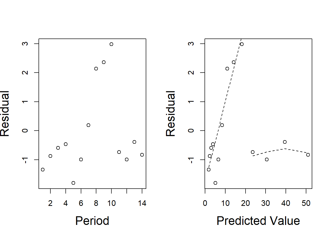
Figure 4.2: Residual plots for the AIDS data. The scatter is reasonably constant around the fine dotted line suggesting that the mean is wrongly specified, but the Poisson error structure could be correct.
The plot of these for the AIDS model is shown in Figure 4.2. It shows why the model does not fit particularly well. Closer examination of the residuals shows that two separate curves could be drawn through the points with reasonably constant variability. Perhaps there are two separate growth processes operating.
The contribution each point makes to the deviance leads to a different form of residual, the deviance residual. Following Equation (4.10) the deviance residual for the Poisson model is
\[\begin{equation} r_D = \left[ 2\left( y_i \ln(y_i/\hat{\mu}_i) - (y_i - \hat{\mu}_i)\right)\right]^{0.5} \tag{4.12} \end{equation}\]
with the same sign as \((y_i - \hat{\mu}_i)\). These are the preferred
form of residual for GLMs because they are directly related to the
amount of influence a point has on the estimates. However residual plots
usually look much the same regardless of the form of residual used. You
can obtain the deviance residuals using the residuals() command
without specifying the type because this is the default type to use.
Note that the sum of the squared deviance residuals is the total
deviance for the model.
Standardisation gives constant variance, but not a normal distribution. The Poisson distribution for example has a very skew distribution and the values can only take integer values. Residual plots can therefore have an unusual appearance, as was shown by plots in Chapter 3.
4.8 Summary
In this chapter we have introduced the generalised linear model via Poisson regression. We have shown how the GLM and iteratively re-weighted least squares methods lead to the same results and parameter estimates. Although it was not explicitly stated at the time, the link function in Example 3.3.1 was the identity, and the distribution was Poisson. \(\frac{\partial \eta}{\partial \mu} = 1\), \(W_i = 1/var(Y_i) = \mu_{(i)} ^{-1}\) and \(z_i = y_i\). With these substitutions the procedure used there becomes the maximum likelihood procedure described in this chapter. We have also introduced use of the log link for Poisson data in the examples in this chapter.
A crucial notion for all GLMs that was covered in this chapter is the deviance. The deviance \(= 2 \ell(\boldsymbol{\beta}_{\max}) - 2 \ell(\hat{\boldsymbol{\beta}})\) behaves like a residual sum of squares. Changes in it as parameters are added to or deleted from the model can be assessed for significance using ratios of mean deviances, which give approximate F-tests.
In Poisson regression, the deviance of the true model has an approximate \(\chi^2\) distribution because there is no scale parameter for the Poisson distribution. We have also seen how the deviance can be evaluated using this result.
4.9 Exercises
- The dataset
RiverProbAllgives the number of problems experienced by travelers on the Whanganui river. This is the full data set including the craft type as a categorical variable. Fit a generalised linear model to this data using a Poisson distribution for the number of problems and a log link function. Use comparisons of the deviance to make any simplifications to a full model you find possible.
This exercise could be used as an in-class tutorial.
- Example 3.3.1 used a subset of the Whanganui river data for Other craft. An identity link was used in that analysis instead of a log link. Calculate the predicted number of problems for a range of river flows using this model, and compare with the predictions for the same flow and Other craft type for the model in Exercise 1 above. Compare the models using a graph.
This exercise could be used as an in-class tutorial.
- There is an assumption when we use the Poisson distribution that all observations come from an equivalent “area of opportunity", but we do not know how many craft are successfully traversing the river at any given flow rate. What consequences does this have on the analyses presented here? N.B. This is a discussion problem and does not require any data analysis.
A note on the Newton Raphson method
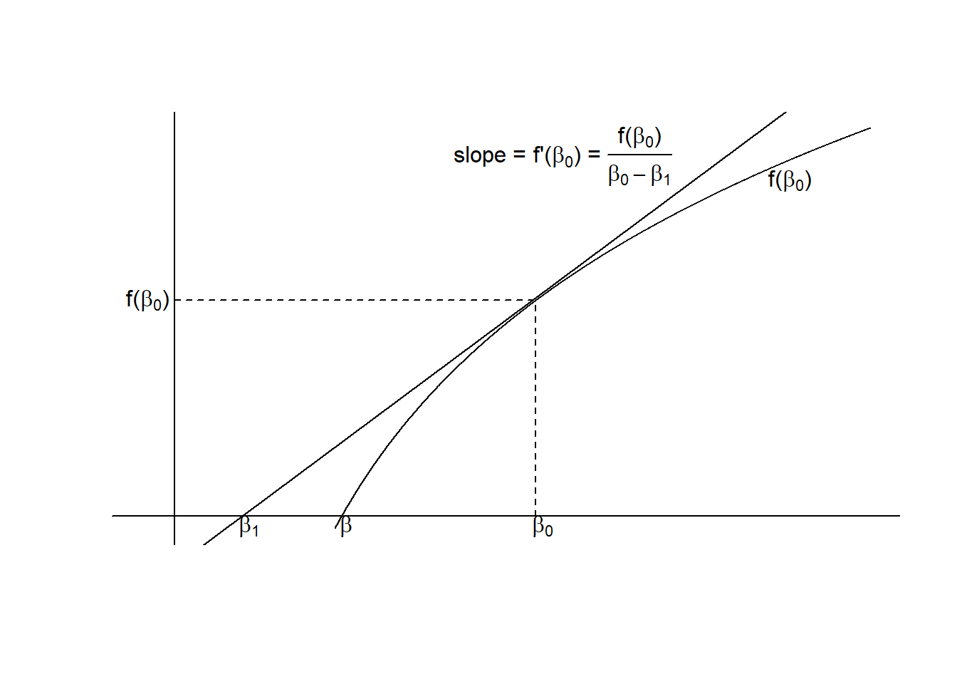
Figure 4.3: Demonstration of the Newton Raphson formula for solving \(f(\beta)=0\). \(\beta_1\) is a better approximation than \(\beta_0\).
The method used is the Newton-Raphson method, which can be understood from the graph in Figure 4.3. Clearly if \(\beta_{(0)}\) is an approximate solution to \(f(\beta) = 0\), \(\beta_{(1)}\) will be a better one. A little calculus and trigonometry gives \(\beta_{(1)}\) in terms of \(\beta_{(0)}\). The derivative of f at \(\beta_{(0)}\) equals the slope of the tangent line, so \[f'(\beta_{(0)}) = \frac{\partial f(\beta)}{\partial \beta} = \frac{f(\beta_{0})}{\beta_{0}-\beta_{1}}\] Rearranging gives the general Newton-Raphson formula for finding the next approximation to a solution:
\[\begin{equation} \beta_{(1)} = \beta_{(0)} - \frac{f(\beta_{0})}{f'(\beta_{0})} \tag{4.13} \end{equation}\]
In our case, from Equation (4.7)
\[f(\beta) = -\frac{\partial l}{\partial \beta} = \sum_{t} { t(e^{\beta t} - y_{t})} = \sum_{t} {t(\hat{\mu}_{t} - y_{t})}\] and \[\frac{\partial f(\beta)}{\partial \beta} = -\frac{\partial^{2} l}{\partial \beta^{2}} = \sum_{t} {t(t e^{\beta t})} = \sum_{t} { t^{2}e^{\beta t}} = \sum_{t}{ t^{2}\hat{\mu}_{t}}\] which when substituted in Equation (4.13) gives
\[\begin{align} \beta_{(1)} & = & \beta_{(0)} - \frac{\sum_{t} {t(\hat{\mu}_{t} - y_{t})}} {\sum_{t} { t^{2}\hat{\mu}_{t}}} \nonumber\\ & = & \frac{\sum_{t} { \hat{\mu}_{t} t \left( t\beta_{0} - 1 + \frac{y_{t}}{\hat{\mu}_{t}}\right)}}{\sum_{t} { t^{2}\hat{\mu}_{t}}} \tag{4.14} \end{align}\]
Now this may not look a particularly familiar expression, but if the model \(z_{t} = \beta x_{t}\) were fitted using weighted least squares with weights \(w_{i}\) the estimate of \(\beta\) would be
\[\begin{equation} \hat{\beta} = \frac{\sum {w_t x_t z_t }}{\sum { w_t x^{2}_{t}} } \tag{4.15} \end{equation}\]
If the following values are substituted into Equation (4.15)(above)
\[\begin{aligned} w_{t} & = & e^{\beta_{(0)} t} = \hat{\mu}_{(0)t} \nonumber\\ x_{t} & = & t \nonumber\\ z_{t} & = & \beta_{(0)}t - 1 + \frac{y_t}{\hat{\mu}_t} = \hat{\eta}_{(0)t} + \frac{y_t - \hat{\mu}_{(0)t}}{\hat{\mu}_{(0)t}} \end{aligned}\] this weighted least squares formula for \(\hat{\beta}\) is exactly the same as Equation (4.13), the formula for \(\beta_{1}\) above, and is the same procedure found empirically earlier (Equation (4.5)).