Chapter6 The Generalised Linear Model for Other Distributions
Chapter Aim: To introduce a model which permits the response variable to have (almost) any continuous distribution, with a mean value equal to (almost) any function of a linear combination of predictor variables; to cater for discrete response variables that do not follow a Poisson or binomial distribution.
6.1 The general case
All the calculations presented in Chapters 4 and 5 can be completed quite generally. For most common distributions the fitting procedure reduces to:
Use the data itself as the starting value \(\hat{\boldsymbol{\mu}}_{(0)}\) perhaps modified to avoid \(\ln(0)\).
Calculate \(\hat{\boldsymbol{\eta}}_{(0)} = g(\hat{\boldsymbol{\mu}}_{(0)})\), \(\boldsymbol{z} = \hat{\boldsymbol{\eta}}_{(0)} + (\boldsymbol{y}-\hat{\boldsymbol{\mu}}_{(0)}) \cdot \frac{\partial\eta_{i}}{\partial\mu_{i}}\) and weights \(\boldsymbol{w}^{-1} = \left( \frac{\partial\eta_{i}}{\partial\mu_{i}} \right)^{2} \cdot var(\boldsymbol{Y})\)
Fit \(\boldsymbol{z}\) to \(\boldsymbol{X}\) using \(\boldsymbol{w}\) as weights, which gives \(\hat{\mu}_{(1)}\)
Then iterate until there is no further change in \(\hat{\mu}\).
On several occasions results have been stated to hold for most distributions. What does ‘most’ mean? The iterative algorithm will work and the estimators will have the asymptotic distributions for all distributions belonging to what is called the exponential family, that is those whose probability functions can be written in the form
\[\begin{equation} f(y) = \exp\left( \frac{ y\theta - b(\theta)}{ a(\phi)} + c(y,\phi)\right) \tag{6.1} \end{equation}\]
This representation of the exponential family definition is known as the natural exponential family. Other representations do exist, and not all members of the full exponential family are easily fitted using the generalised linear model framework. For example, (Thurston et al. 2000) state that the negative binomial distribution is not in the exponential family, but what they actually mean is that the negative binomial distribution cannot be expressed in the form of Equation (6.1).
The most familiar members of this family are the Poisson, binomial, gamma and normal but others do exist. For this family \(E(Y) = \mu = b^\prime (\theta)\) and \(var(Y) = b^{\prime \prime} (\theta)a(\phi)\).
As an example, for the Poisson distribution \(a(\phi) = 1\), \(b(\theta) = e^{\theta}\), and \(c(y,\phi) = -\ln(y!)\). Substituting these into Equation (6.1) gives \[\begin{aligned} f(y) & = & \exp\left( (y\theta - e^{\theta}) -\ln(y!) \right) \nonumber\\ & = & \frac{ \left(\exp(\theta )\right)^y \exp(-e^{\theta })}{y!}\end{aligned}\] Substituting \(e^{\theta} = \lambda\) gives the familiar Poisson density: \[f(y) = e^{-\lambda}\frac{\lambda^{y}}{y!}\] And \(\mu = b^\prime (\theta) = e^{\theta} = \lambda\), \(\sigma^2 = b^{\prime\prime}(\theta)a(\phi) = e^{\theta} = \lambda\), familiar results for the Poisson distribution.
For the normal distribution, \(a(\phi) = \phi=\sigma^2\), \(b(\theta) = \theta^2/2\) (\(\theta=\mu\)), and \(c(y,\phi) = \frac{-1}{2} \left( \frac{y^2}{\phi} + \ln(2\pi\phi) \right)\). Checking that this gives the correct mean and variance is left as an exercise.
6.2 Quasi-likelihood — An empirical approach
Quite often the Poisson or binomial distributions might seem appropriate but the variance is too large (or small). That is \(a(\phi)\) from Equation (6.1) should be 1, but is not. Since the distribution of Y enters the iterative procedure only to specify \(var(Y)\) as a function of \(\mu\), may we use the procedure if all that is known about the distribution is \(var(Y)\)? For example if the response is a proportion based on a continuous variable rather than a binomial count the variance might still be proportional to \(p(1-p)\), but the binomial, which is discrete, is in no way the correct distribution. Could we use the proportion, telling the computer that it was a binomial random variable with \(n =1\)? Or use a percentage as a binomial with \(n =100\)?
More generally if data plots suggest that \(var(Y_i) = \phi var(\mu_{i})\) may we use \(var(Y_i) = var(\mu_{i})\) in the iterative algorithm, estimate \(\phi\), and thereby get sensible estimates of \(\beta\)?
Firstly, \(\phi\), often called the dispersion (a measure of how spread out the data is), is best estimated as
\[\begin{equation} \sum {\left\{(y_{i} - \hat{\mu}_{i})^{2}/(n - p)var(\hat{\mu}_{i})\right\} } \tag{6.2} \end{equation}\] where \(n\) is the sample size and \(p\) is the number of regression coefficients that need to be estimated.
Although these estimates of the parameters and means are sensible, because they are not based on a likelihood function they cannot be guaranteed to have the asymptotic properties of maximum likelihood estimates. This is discussed in more detail in the next section, but pragmatically no small sample inferences can be regarded as exact with generalised linear models, and what is ‘small’ gets bigger the further the truth moves from the justifying theory.
Computer programs provide a choice. The simple option is based on the generalised model as described in Section 4.1, where a standard distribution and link function are specified. There will however be a more advanced option, the quasi-likelihood option, providing a range of functions specifying the variance as a function of the mean.
6.3 The Generalised Linear Model for a Gamma distribution
It was stated above (without proof) that the gamma distribution is a member of the exponential family that can be expressed in the natural form. The probability density function of the gamma distribution is
\[f(x; a, b) = \frac{a(ax)^{b-1} e^{-ax}}{\Gamma(b)}\] where \(x,a,b>0\).
The distribution is called the Erlang distribution when the shape parameter is integer \((b \in \mathbb{N)}\), and when \(b=1\) the gamma reduces to the exponential distribution. It is therefore a very useful distribution for model-fitting purposes. Note that \(\Gamma(b)\) is known as the gamma function of b.
6.3.1 Example: Clotting times of blood
| Concentration (%) | Agent 1 | Agent 2 |
|---|---|---|
| 5 | 118 | 69 |
| 10 | 58 | 35 |
| 15 | 42 | 26 |
| 20 | 35 | 21 |
| 30 | 27 | 18 |
| 40 | 25 | 16 |
| 60 | 21 | 13 |
| 80 | 19 | 12 |
| 100 | 18 | 12 |
The table 6.1 shows the mean clotting times (y) in seconds of blood for nine percentage concentrations (x) of normal plasma and two lots of clotting agent.
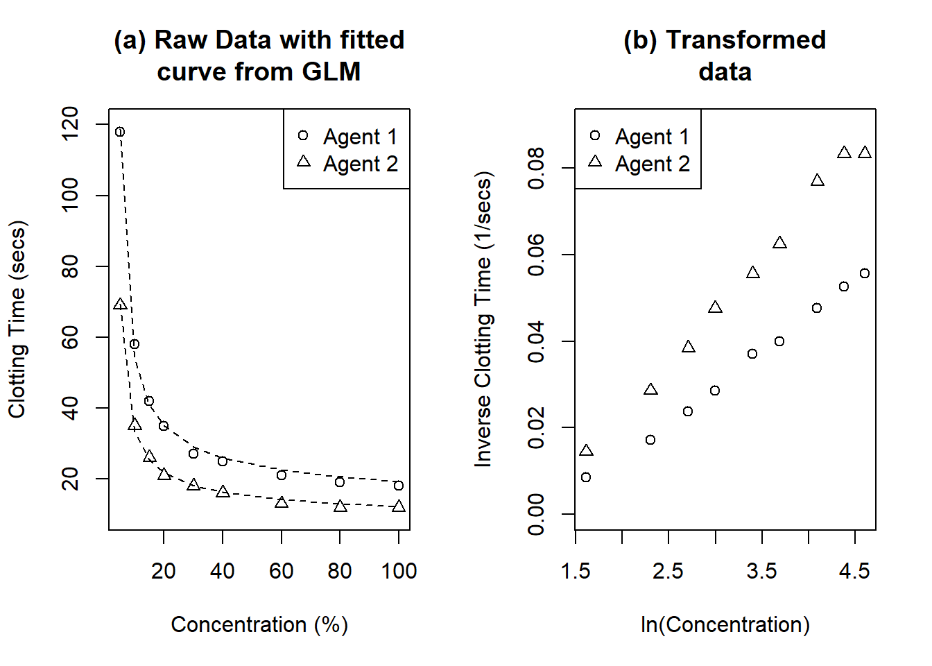
Figure 6.1: Clotting time of blood with nine concentrations of normal plasma and two clotting agents. (a) shows the raw data with fitted curves from GLMs. (b) shows the transformed data. The GLMs fitted in (a) would be analogous to straight lines in (b).
The data is plotted in Figure 6.1. Plot (a) looks a little like a rectangular hyperbola, which suggests fitting \[\frac{1}{y} = ax + b\] Plot (b) shows \(1/y\) against \(\ln x\), which does look a moderately good fit to a straight line. Using \(1/y\) is equivalent to replacing the time to clot with the rate of clotting. Apparently the plasma concentration is related linearly to the rate of clotting rather than the time of clotting, which does sound reasonable.
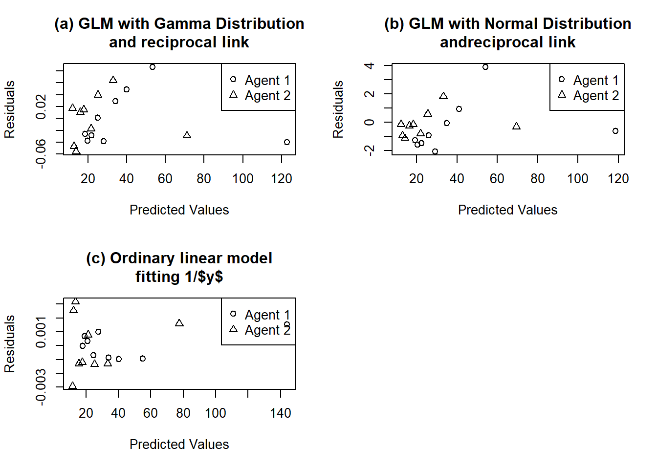
Figure 6.2: Residual plots for blood clotting data. (a) GLM with Gamma distribution and reciprocal link. (b) GLM with normal distribution and reciprocal link. (c) Ordinary linear model fitting 1/\(y\).
The variability of \(1/y\) does not appear constant, however, and nor does the variability of y . Residuals are plotted in Figure 6.2. In fact the variability of y appears to increase with the mean of y. The standard deviation of the gamma distribution is proportional to the mean, which suggests using the gamma as the error distribution. Fitting a gamma distribution with reciprocal link gives the results shown in Table 6.2. The large ratios (equivalent to F ratios) show that each term is significant.
Different programs give different forms of these parameter estimates. Typical output is shown in Table 6.2.
    time=c(118,58,42,35,27,25,21,19,18,69,35,26,21,18,16,13,12,12)
    agent=as.factor(c(rep("Agent1",9),rep("Agent2",9)))
    concentration=rep(c(5,10,15,20,30,40,60,80,100),2)
    full.glm = glm(time~agent*log(concentration),family=Gamma(link="inverse"))
    anova(full.glm,test="F")
summary(full.glm)| Df | Deviance | Resid. Df | Resid. Dev | F | Pr(>F) | |
|---|---|---|---|---|---|---|
| NULL | 17 | 7.709 | ||||
| agent | 1 | 1.077 | 16 | 6.631 | 505.8 | 2.18e-12 |
| log(concentration) | 1 | 6.331 | 15 | 0.300 | 2972.7 | 1.04e-17 |
| agent:log(concentration) | 1 | 0.271 | 14 | 0.029 | 127.3 | 2.06e-08 |
| Estimate | Std. Error | t value | Pr(>|t|) | |
|---|---|---|---|---|
| (Intercept) | -0.016554 | 0.000865 | -19.127 | 1.97e-11 |
| Agent2 | -0.007354 | 0.001678 | -4.383 | 0.000625 |
| ln(concentration) | 0.015343 | 0.000387 | 39.626 | 8.85e-16 |
| Interaction | 0.008256 | 0.000735 | 11.228 | 2.18e-08 |
These represent fitting a line to Agent 1, then adding the differences between Agent 1 and Agent 2. So the constant for Agent 2 is: \[Intercept + Agent \, 2 = -0.016554 - 0.007354 = -0.023908\] And the slope for Agent 2 is \[Slope + interaction = 0.015343 + 0.008256 = 0.023599\] The fitted model is equivalent to two lines: \[\begin{array}{rcl} \textrm{Agent 1:} & (mean \, time)^{-1} & = -0.016554 + 0.015343x \\ \textrm{Agent 2:} & (mean \, time)^{-1} & = -0.023908 + 0.023599x \end{array}\]
Note the similarity with the very first example in Chapter 1, comparing baby’s birth weights.
What makes this example different from the Poisson example is that the gamma distribution has a scale parameter. If the chosen model is correct it can be shown that the mean residual deviance is an estimate of \(var(Y/\mu) = var(Y)/\mu^2\), or the square of the coefficient of variation, which is constant. Here the mean deviance is (/), giving an estimate of \(\sqrt{0.0021} = 0.046\) for \(\sigma / \mu\) , the coefficient of variation. The standard deviation is therefore 4.6% of the mean. The deviance is \(2 \sum {\left[ \ln\left( \frac{y_i}{\hat{\mu}_i} \right) - \frac{y_i - \hat{\mu}_i}{\hat{\mu}_i} \right]}\), so if any observations are very small (i.e. \(\hat{\mu}\) small) they will also be very influential.
Although the analysis parallels normal theory linear models closely, you must always remember that the true distributions are only roughly chi-squared, and the conventional tests are only a guide to how well the model fits.
6.4 Summary
The derivation in the maximum likelihood discussion of Section 4.4 applies to any generalised linear model.
We have
\[\begin{align} \eta_i & = \boldsymbol{\beta}^T \boldsymbol{x}_i & \notag \\ E(Y_i) & = \mu_i & = g^{-1}(\eta_i ) \tag{6.3} \end{align}\]
and the density function of \(y_i\), \(f(y_i)\)
Then the log-likelihood function is
\(\ell(\boldsymbol{\beta}) = \sum {\ln \left( f(\boldsymbol{\beta};y)\right)}\).
Maximum likelihood estimates of \(\boldsymbol{\beta}\) are found by solving \[\frac{\partial \ell(\boldsymbol{\beta})}{\partial \beta_i} = 0\] for each \(\beta_i\).
These equations need to be solved iteratively using the Newton-Raphson method. That is, if \(\boldsymbol{\beta}_{(m)}\) is the mth approximation to \(\boldsymbol{\beta}\), \[\boldsymbol{\beta}_{(m+1)} = \boldsymbol{\beta}_{(m)} - \left[ \frac{\partial^2 \ell}{\partial \beta_j \partial \beta_k } \right]^{-1}_{\boldsymbol{\beta} = \boldsymbol{\beta}_{(m)}} \left[ \frac{\partial \ell}{\partial \boldsymbol{\beta}} \right]_{\boldsymbol{\beta} = \boldsymbol{\beta}_{(m)}}\] These equations can be shown to reduce to the weighted least squares equations \[\boldsymbol{X}^T\boldsymbol{W}\boldsymbol{X}\boldsymbol{\beta}_{(m+1)} = \boldsymbol{X}^T\boldsymbol{W}\boldsymbol{z}\] where \[z_i = \boldsymbol{x}^T_{i} \boldsymbol{\beta}_{(m)} + (y_i - \hat{\mu}_i )\frac{\partial \eta_i}{\partial \mu_i}\] and \[\boldsymbol{W} = \textrm{diag} \left\{ \frac{1}{var(Y_i)} \left[ \frac{\partial \eta_i}{\partial \mu_i} \right] ^{-2} \right\}\] The next approximation to \(\boldsymbol{\beta}\) can therefore be found by a standard weighted regression of \(\boldsymbol{y}\) against \(\boldsymbol{z}\) using \(\boldsymbol{w}\) as weights.
We have now seen that the GLM framework is used for many distributions. The exponential family was introduced and its most common members have now been used in examples of the GLM.
We now know that if the response variable’s distribution is able to be expressed in the natural form of the exponential family, we could either use the GLM procedures available in statistical software, or write a iteratively re-weighted least squares procedure of our own design to meet our needs.
6.5 Exercises
- Wedderburn’s leaf blotch data (Hardin and Hilbe 2012) represents the proportion of leaf blotch on ten varieties of barley grown at nine sites in 1965. The amount of leaf blotch is recorded as a percentage. Obtain the data using:
and answer the following questions.
1.  obtain the data and check that variety and site are correctly
defined.
2.  fit a GLM that is appropriate for this data, assuming the data are
binomially distributed.
3.  Why can't we fit the interaction model here.
4.  produce a plot of the residuals vs the predicted values for this
model and identify any problems that might exist.
5.  fit the following model.
Leaf.glm.quasi = glm(Prop~Site+Variety, family=quasibinomial(), data=LeafBlotch, weights=rep(100, nrow(LeafBlotch)))
6.  produce a plot of the residuals vs the predicted values and identify
if this is a better option than using the previous model.
7.  What is the dispersion parameter for this model?
8.  Describe the effect site and variety have on the proportion of leaf
blotch.
This exercise could be used as an in-class tutorial.
- Investigate the car insurance claims data, used by (McCullagh and Nelder 1989). Obtain the data using:
Your task is to model the average claims (AveClaim) for damage to an owner’s car on the basis of the policy holder’s age group (AgeGroup
1-8), the vehicle age group (VehicleAge 1-4), and the car group
(CarGroup 1-4). Be sure you check if any of the two-way interactions are
significant.
Hint use glm with family=gamma() and link="inverse"
This exercise could be used as an in-class tutorial.
- predict patient survival in a Drug trial based on age and type of drug. Obtain the data using:
Fit a GLM compare the use of link=log to link=identity.
This exercise could be used as an in-class tutorial.
- The `MASS package includes a dataset that kills snails under experimental conditions.
We will use it to compare binomial and quasibinomial models.