Chapter3 Weighted Regression with Iteration
Chapter Aim: To introduce the idea of using iterative fitting with estimated weights as a way of fitting models to response variables where the variance depends on the mean.
3.1 Theoretical background
3.1.1 Gauss Markov theorem
The justification for least square methods is the Gauss Markov theorem, which states that amongst unbiased linear estimators the least square estimator has minimum variance. For this to be true the dependent variables (Y) must all be uncorrelated and must have equal variances. That is, \(var(Y_i) = \sigma^2\) for all i. Note that this theorem makes no assumption about the distribution of the Y, and also note that transformations introduce a nonlinear component into estimation.
Because there is no assumption about the distribution of the response variable the Gauss Markov theorem is very powerful. The rationale for an even spread of residuals in residual plots is that an even spread indicates a constant variance, which in turn indicates that estimators will have minimum variance. If the variances are not equal there is a generalisation of the Gauss Markov theorem. If the variances of the Y’s are known, that is \(var(Y_i) = \sigma^2/w_i\), then weighted least squares, using \(w_i\) as the weight for each observation, gives the minimum variance linear estimators.
The actual procedure is to write \[\begin{aligned} Y^{*}_i &=& w^{1/2}_i Y_i \\ x^{*}_i &=& w^{1/2}_i x_i \\\end{aligned}\] then \[var(Y^{*}_i) = var(w^{1/2}_i Y_i ) = w_i var(Y_i) = \sigma^2\] and \[Y^{*}_i = w^{1/2}_i Y_i = w^{1/2}_i \boldsymbol{\beta}^T \boldsymbol{x}_i = \boldsymbol{\beta}^T \boldsymbol{x}^{*}_i\] so that the standard linear model applies to \(Y^{*}_i\) and \(\boldsymbol{x}^*_i\), and the Gauss Markov theorem applied to \(Y^{*}_i\) tells us that the weighted least squares estimate of \(\boldsymbol{\beta}\) is of minimum variance.
3.1.2 Weighted regression
In Chapter 2, transformations were used to achieve constant variance, but they also change the relationship between \(\mu_{Y_i}\) and \(\boldsymbol{\beta}^T \boldsymbol{x}_i\). By using weights different variances can be accommodated independently of the relationship between \(E[Y]\) and \(\boldsymbol{x}\), and we no longer need to search for a transformation which simultaneously achieves two independent goals. The serious catch is that the variances are usually unknown. There are three not entirely exclusive possibilities. Sometimes there are several observations for each \(\boldsymbol{x}_i\) from which an estimate of the variance can be made. The deer example, Example 1.5.1, illustrated this method. Unfortunately good estimates of the variance require large samples and these are very rarely available.
Much more often the variability can be modelled as a function of the mean of Y. That is \[var(Y_i) = \sigma^{2}f ( \mu_{Y_i } )\] and the \(w_i\) are all replaced with \(1/f(\mu_{Y_i })\). The actual form of f might be determined empirically. Even if there are only duplicate observations for each \(\boldsymbol{x}\), combining information over all of them often permits a reasonable guess at the form of f. Note that the weights need only be determined proportionately because any constant is absorbed into \(\sigma^{2}\) which is estimated anyway. In Chapter 2 a method was described for finding a transformation to stabilise the variance for any given f.
The third possibility, and it is the one which leads into generalised linear models, is the case where Y has a distribution whose variance is a function of its mean. The simplest case is the Poisson, and that is the subject of Example 3.2.1.
3.2 Iteratively reweighted least squares
3.2.1 Example: An Artificial Example
The data in Table 3.1 shows an artificial example.
|
|
|
The plot in Figure 3.1 suggests that the spread of the points is increasing not quite in proportion to \(\mu_{Y}\).
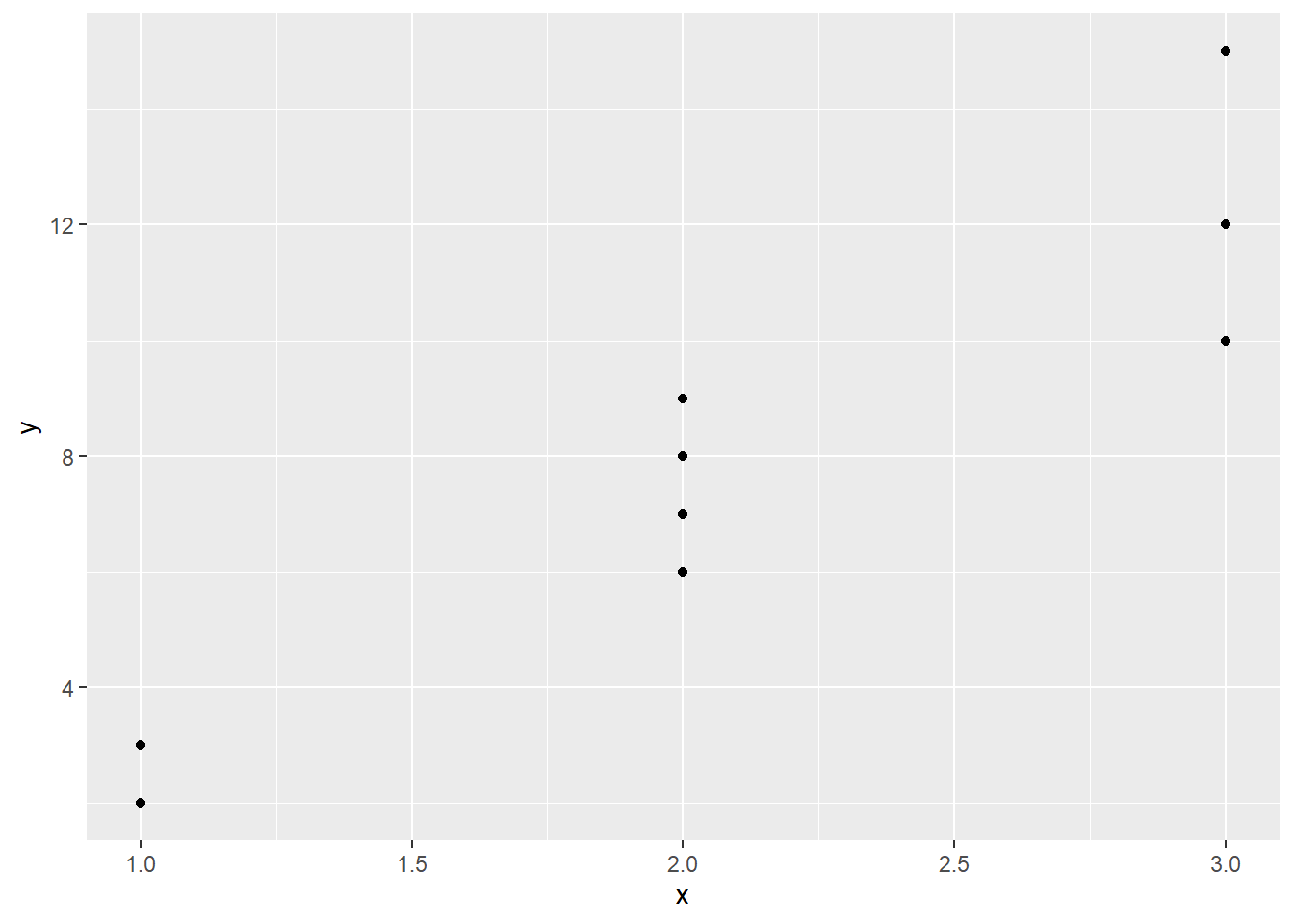
Figure 3.1: Artificial data plotted.
Perhaps the variance is proportional to the mean suggesting that the response follows a Poisson distribution (\(\sigma^2=\mu=\lambda\) for the Poisson). If a square root transformation were used to stabilise the variance (see Chapter 2), the linear relationship between \(\mu_{Y}\) and x would be lost.
The model needed is: \[\begin{aligned} \mu_{Y_i } & = & \beta_{1} + \beta_{2} x_i \nonumber \\ var(Y_i) & = & k \mu_{Y_i }\end{aligned}\] But the \(\mu_i\) are unknown, and cannot even be estimated without estimates of the \(\beta\)’s. And the original aim was to obtain estimates of the \(\beta\)’s which weighted the Y’s according to their variance, \(\mu\). The resolution of this Catch 22 lies in proceeding iteratively.
First, forget about weights and just estimate an ordinary regression line of y on x.
Call:
lm(formula = y ~ x, data = Artificial)

Residuals:
   Min     1Q Median     3Q    Max
-2.364 -0.545 -0.364  0.545  2.636

Coefficients:
            Estimate Std. Error t value Pr(>|t|)
(Intercept)   -2.364      1.630   -1.45  0.19028
x              4.909      0.729    6.73  0.00027 ***
---
Signif. codes:  0 '***' 0.001 '**' 0.01 '*' 0.05 '.' 0.1 ' ' 1

Residual standard error: 1.61 on 7 degrees of freedom
Multiple R-squared:  0.866, Adjusted R-squared:  0.847
F-statistic: 45.4 on 1 and 7 DF, p-value: 0.000269Predictions=predict(ModelU)
Beta0<-coef(ModelU)[1]
Beta1<-coef(ModelU)[2]
RMS<-sum(resid(ModelU)^2/ModelU$df)
Results<- c(Beta0, Beta1, RMS)The equation of this line is: \[y = -2.364 + 4.909 x\]
This equation can be used to give estimates of the \(\mu_i\) as \(\hat{y}_i\), shown in Figure 3.2
Artificial =     Artificial  |> mutate(PredictionsU =Predictions)
Artificial |> ggplot(aes(x=x, y=y)) + geom_point() + geom_point(aes(y=PredictionsU), col="red") 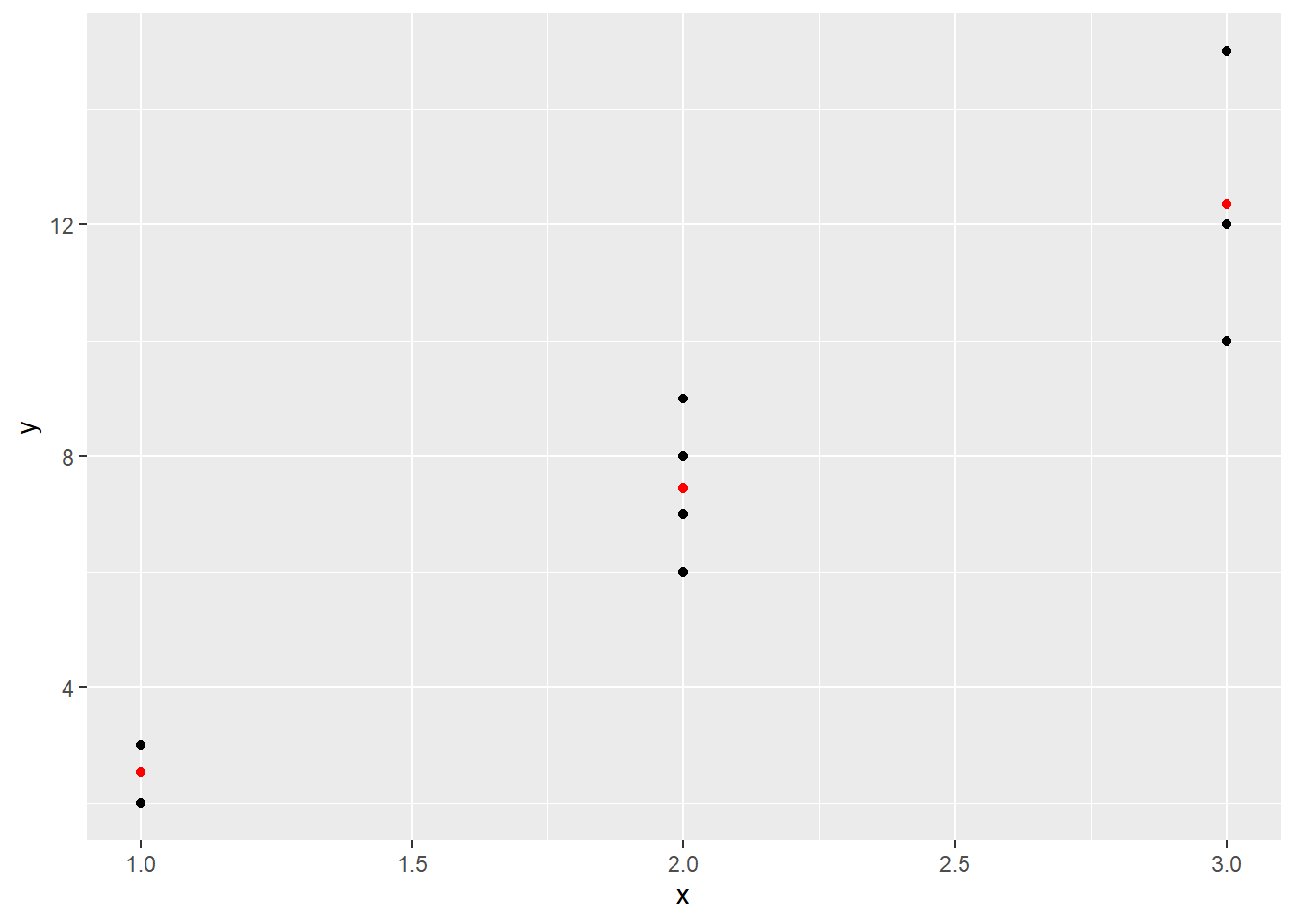
Figure 3.2: Raw observed data (black) and predictions from an unweight model (red).
These values of \(\mu_i\) provide estimates of \(var(Y_i)\) to be used in a weighted regression of y on x, giving new, hopefully better, estimates of \(\beta_{0}\) and \(\beta_{1}\), and hence better estimates of \(\mu_i\).
The first weighted model (the first iteration):
ModelW <-update(ModelU, weights=1/Predictions)
Predictions=predict(ModelW)
Beta0<-coef(ModelW)[1]
Beta1<-coef(ModelW)[2]
RMS<-sum(1/predict(ModelW)*resid(ModelW)^2/ModelW$df)
Results<-rbind(Results, c(Beta0, Beta1, RMS))
and the second iteration:
ModelW <-update(ModelW, weights=1/Predictions)
Predictions=predict(ModelW)
Beta0<-coef(ModelW)[1]
Beta1<-coef(ModelW)[2]
RMS<-sum(1/predict(ModelW)*resid(ModelW)^2/ModelW$df)
Results<-rbind(Results, c(Beta0, Beta1, RMS))
The second iteration’s code should be repeated until the \(\beta\)’s and therefore the \(\mu\)’s converge to stable values. Adding a “loop” to get the iterations going gives the following code:
for(i in 1:3){
    ModelW <-update(ModelU, weights=1/Predictions)
    Predictions=predict(ModelW)
    Beta0<-coef(ModelW)[1]
    Beta1<-coef(ModelW)[2]
    RMS<-sum(1/predict(ModelW)*resid(ModelW)^2/ModelW$df)
    Results<- rbind(Results, c(Beta0, Beta1, RMS))
    }
This code builds tables of predicted values as well as results for the model coefficients and residual mean squares. Figure 3.3 shows the first simple regression line and the line the process converges to.
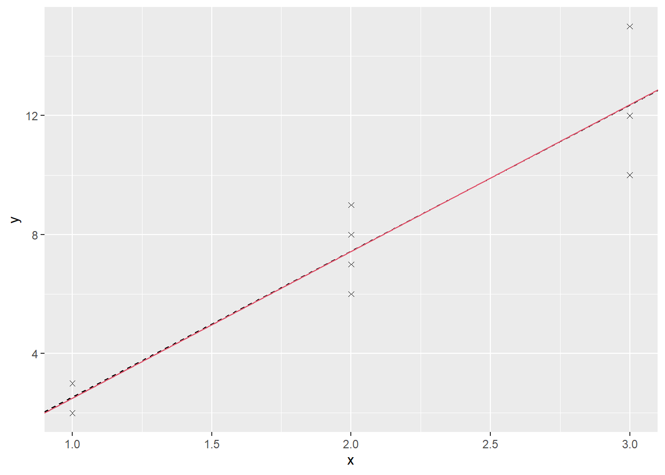
Figure 3.3: Fitted lines from the unweighted (black) and weighted (red) models for the Artificial data.
At first sight there may seem to be only one line, but this is because the final one is almost the same as the first: \[y = -2.419 + 4.935 x\] Table 3.2 shows how the values for the model change over the first few iterations.
| Intercept | Slope | RMS | |
|---|---|---|---|
| Results | -2.364 | 4.909 | 2.5974 |
| -2.419 | 4.935 | 0.2706 | |
| -2.419 | 4.935 | 0.2706 | |
| -2.419 | 4.935 | 0.2706 |
We also know that the value of RMS (the weighted sum of squares
divided by degrees of freedom) links the variance of the Y’s to the
\(\mu_Y\): \[RMS = \frac{\sum{w_i (y_i - \hat{y}_i)^2 }}{n - p}\] or,
for our scenario: \[var(Y) = 0.271 \mu_Y\]
3.2.2 Residuals
The raw residuals \(y_i -\hat{\mu}_i\) can be approximately standardised by dividing them by their estimated standard deviations, but neither the raw or standardised residuals are appropriate for validating a weighted regression model.
In weighted regression models, we calculate residuals that reflect the weights used in the model. The process is a kind of standardisation in that we divide the residual by its estimated standard deviation, which is usually the square root of the reciprocal of the weight used for the corresponding observation. For weights based on having a Poisson distribution for \(y_i\) we multiply by \(\sqrt{W_i }\) which is the same as dividing by \(\sqrt{\hat{\mu}_i}\).
The resulting values, sometimes called Pearson residuals, should behave like residuals from a standard linear model in the residual plots, providing a check on the original assumption (in this example) that the distribution is Poisson. Figure 3.4 shows both sets of residuals plotted.
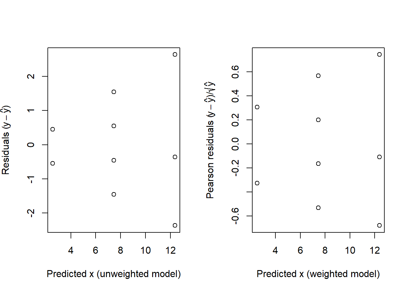
Figure 3.4: Raw residuals for the unweighted model (left) and the Pearson residuals for the weighted model, both plotted against the corresponding fitted values.
For a standard linear model created using the lm() command, the
default action of the residuals() command is to obtain raw residuals.
An alternative to using the argument here is to use the specific command
in place of the general residuals() command.
A further property of the residuals in this case is that because \(var(Y_i) = \mu_i\) the constant k should be 1.0, which implies that the RMS of the ANOVA table has an expected value of 1.0 also. In this example the RMS, which was used to estimate k, is 0.271, a little low. In fact the RMS is related to a \(\chi^{2}\) distribution by \[\frac{\mathrm{RMS}\times(\textrm{degrees of freedom})}{\sigma^2} \sim \chi^2_{(\textrm{degrees of freedom})}\]
Here the residual degrees of freedom are 7 and \(\chi^{2}_{7;0.025} = 1.690\) so the lower 95% critical value for testing \(H_0\) that \(\sigma^{2}=1\) is 1.69/7 or 0.241. The actual value of 0.271 just scrapes in.
Iterative processes do not always behave as well as this one. For example, through sampling variability \(\hat{\mu}_i\) could be negative, implying a negative variance. A negative weight will upset many weighted regression computer programs, and could lead to negative sums of squares.
3.3 Difficulties with the procedure
3.3.1 Example: Problems craft have travelling the Whanganui River
In 1988 the Department of Conservation surveyed people travelling down the Whanganui River to find out how river flow levels affected their journey. Travellers were asked at how many rapids they had difficulty. Data for the 21 travellers in craft other than canoes (mainly rafts) is used to plot the number of problems against flow is shown in Figure 3.5.
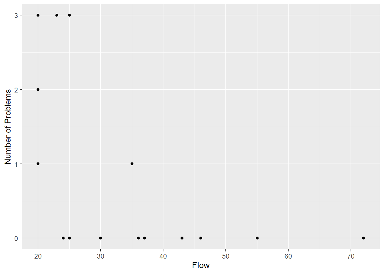
Figure 3.5: The number of problem rapids for 21 travellers on the Whanganui River against the flow level.
On the basis of this graph, you may doubt whether it is worth fitting any model to this data, but it is clear that the variance in number of problems is much higher at low flows than at high flows. Equally clearly, an unweighted, straight line drawn through the points would imply a negative mean number of problems at high flow levels. This is strong evidence that a straight line is not appropriate, but to demonstrate how the weighted procedure can be modified, and to contrast with an alternative model described in Chapter 4, we will fit one nevertheless.
The modification is quite simple. Where a predicted mean is negative, it is changed to a small positive number to provide a positive weight. The outcome of fitting the unweighted model and then the weighted model (using an iterative procedure) is done using the following code:
Model <-lm(Problems~Flow,data=RiverProb)
ModelU = Model
Beta0U<-coef(ModelU)[1]; Beta1U <- coef(ModelU)[2]
RMSU <- sum(resid(ModelU)^2/ModelU$df)
for(i in 1:8){
    Weight <- replace(predict(Model),predict(Model)<=0,0.001)
    Model<-update(Model,weights=1/Weight)
    }
ModelW<-Model
Beta0W<-coef(ModelW)[1]; Beta1W<-coef(ModelW)[2]
RMSW<-sum(1/Weight * resid(ModelW)^2/ModelW$df)
c(Beta0U, Beta1U,RMSU)
(Intercept) Flow
1.8936 -0.0375 1.0239 (Intercept) Flow
1.22329 -0.01703 1.40519 After eight iterations the predicted means converge to give the solid red line shown in Figure 3.6. This line has been forced to pass through the point at a flow of 72 with zero problems, making it a very influential point. The iteration works this way because the near zero predicted mean implies a Poisson distribution with near zero variance, which implies a very large weight. In fact the predicted value at this point is still slightly positive, because a prediction of zero would give an infinite weight.
RiverProb |> ggplot(aes(y=Problems, x=Flow)) + geom_point() + ylab("Number of Problems")+
    geom_abline(intercept=Beta0U, slope=Beta1U, lty=2)+
    geom_abline(intercept=Beta0W, slope=Beta1W, col="red")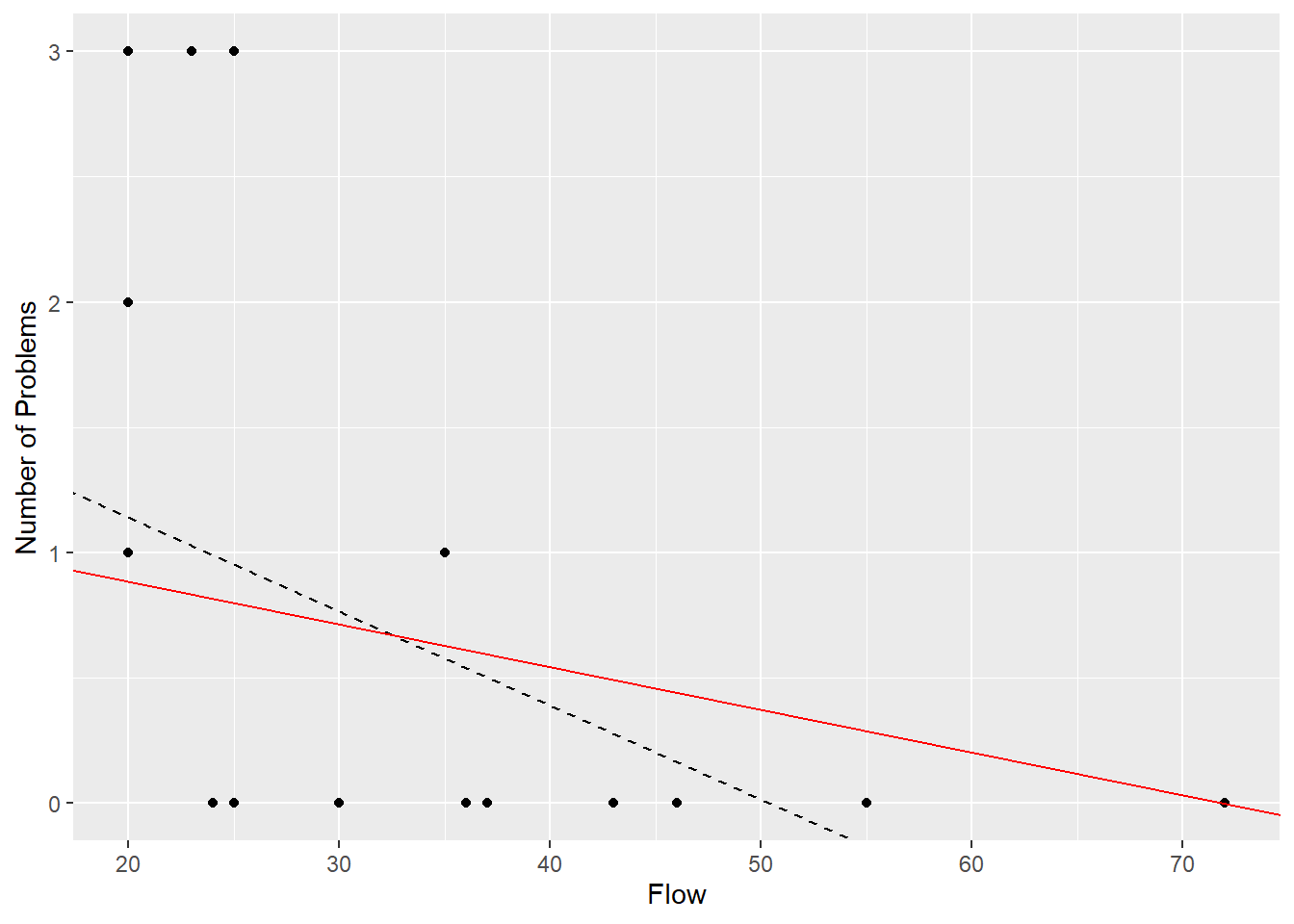
Figure 3.6: Fitted lines for the number of problems versus flow rate, using an unweighted (black) and weighted (red) model.
Figure 3.7 presents the residuals for the unweighted and weighted models.
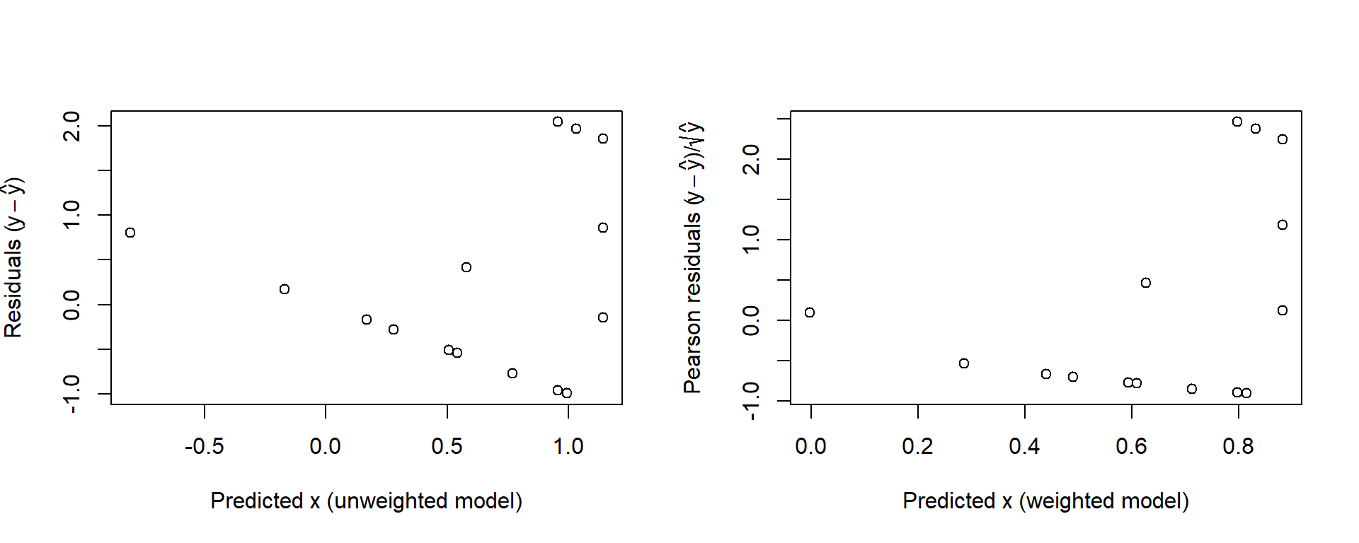
Figure 3.7: Raw residuals for the unweighted model (left) and the Pearson residuals for the weighted model, both plotted against the corresponding fitted values.
3.4 Application to the exponential distribution
3.4.1 Example: Survival time of leukemia patients
The survival time in weeks after blood
cell counts were made on Leukemia patients canbe be found in the Leukemia data included in the ELMER package.
Waiting times to a random event can often be modelled by an exponential distribution. In this the variance is the square of the mean.
Table 3.3 shows the predicted values with no weighting, and the predicted values after iterations have converged.
| Time | Count | PredictionsU | PredictionsW |
|---|---|---|---|
| 65 | 3.36 | 106.024 | 93.33 |
| 156 | 2.88 | 134.639 | 115.30 |
| 100 | 3.63 | 89.928 | 80.98 |
| 134 | 3.41 | 103.044 | 91.04 |
| 16 | 3.78 | 80.986 | 74.11 |
| 108 | 4.02 | 66.679 | 63.13 |
| 121 | 4.00 | 67.871 | 64.05 |
| 4 | 4.23 | 54.160 | 53.52 |
| 39 | 3.73 | 83.967 | 76.40 |
| 143 | 3.85 | 76.813 | 70.91 |
| 56 | 3.97 | 69.659 | 65.42 |
| 26 | 4.51 | 37.468 | 40.71 |
| 22 | 4.45 | 41.044 | 43.45 |
| 1 | 5.00 | 8.256 | 18.28 |
| 1 | 5.00 | 8.256 | 18.28 |
| 5 | 4.72 | 24.948 | 31.10 |
| 65 | 5.00 | 8.256 | 18.28 |
Figure 3.8 suggests that a curve might be more appropriate, and indeed the residual plot does not provide strong evidence that the Pearson residuals \[\label{PearsonResidExp} \frac{y_i - \hat{\mu}_i }{\hat{\mu}_i }\] are more homoscedastic than the raw residuals \[y_i - \hat{\mu}_i\]
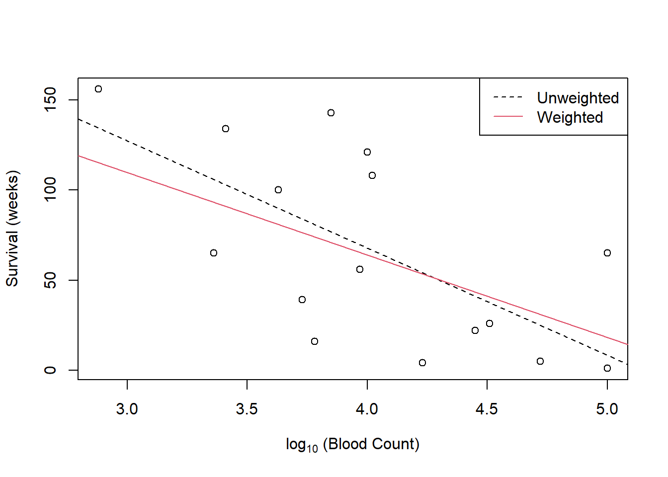
Figure 3.8: Plot of unweighted (lack) and weighted (red) models to the Leukemia data.
The weighted line is less steep, because at low blood counts where the mean survival time is higher the variance is larger and the points have less weight. The line is pulled towards the lower points.
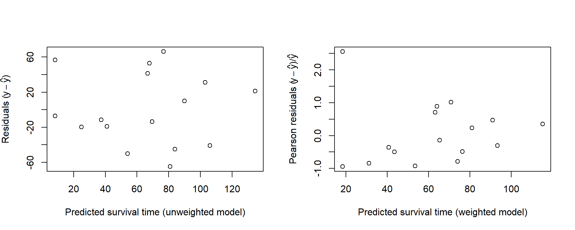
Figure 3.9: Residual plots for the Leukemia data.
3.5 Concluding thoughts
The weight procedure has not been given any strong theoretical justification in this chapter. Remember that the weights, because they have to be estimated, introduce extra variability which is not accounted for in the standard inference procedures. Remember too that the distribution of the residuals, even if standardised, is not normal, again ruling out standard inference procedures without further justification. The step forward was to take account of variance which is not constant but is a function of the mean, without influencing the nature of the relationship between the mean and the explanatory variables.
3.6 Exercises
This exercise could be used as an in-class tutorial.
- A straight line did not model the mean of the river problems in Example 3.3.1 at all well. Try fitting: \[\begin{aligned} \mu_{Y} & = & \beta_0 + \beta_1\ln{x} \\ var(Y) & = &k \mu_Y\end{aligned}\] Compare the fit of this model with the earlier one.
This exercise could be used as an in-class tutorial.
- Fit the model \[\mu_Y = \beta_0 + \beta_1 Dose\] to the beetle mortality data (Example 2.4.1) using iterative reweighting based on Y having a binomial distribution. Compare the predictions with those from the arcsine transformation.