Chapter1 What You Should Know Already
Chapter Aim: To work through some examples to revise applications of the standard linear model.
1.1 Introduction
The linear model as studied in regression papers can be adapted to fit a wide variety of applications. Although the following examples are revision they also introduce terminology and ideas which will be generalised as the course progresses.
1.2 Categorical variables in regression
1.2.1 Example: Birthweight and gestational age for male and female babies.
This example is adapted from (Dobson and Barnett 2008) (pages 23-32). The data in Table 1.1 are the birthweights (g) and estimated gestational ages (weeks) of twelve male and female babies.
|
|
The mean ages are almost the same for both sexes, but the mean birthweight for males is higher than for females.
Graphical discussion
Figures 1.1 to1.5 show scatter plots for the data with the different superimposed lines representing five possible linear models.
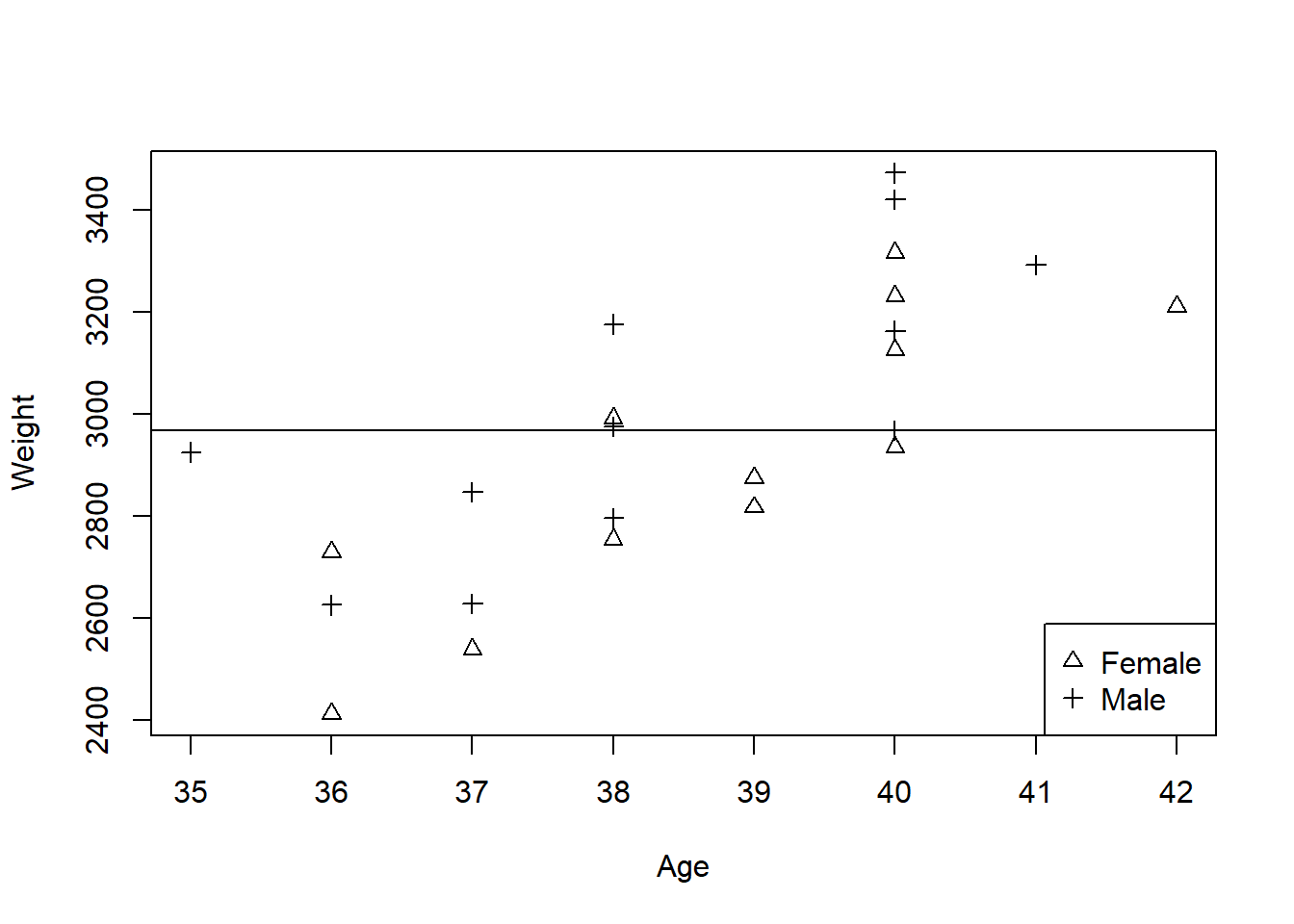
Figure 1.1: Predicted baby weights using only an Overall mean
Figure 1.1 shows a line through the mean and represents a model which says that babies’ weights have nothing to do with their gestational age or their sex. Clearly this is not a realistic model, but it is the basis from which more complex models can be built. The sum of squared residuals from this line is the ‘Total Sum of Squares’ in an analysis of variance table.
Figures 1.2 and 1.3 are both obtained by adding one term to the model depicted in Figure 1.1. If sex alone is in the model, males are different from females, but babies of different gestational ages have the same weight. If age alone is in the model the obvious trend for older babies to be heavier is allowed for, but there are no differences between males and females.
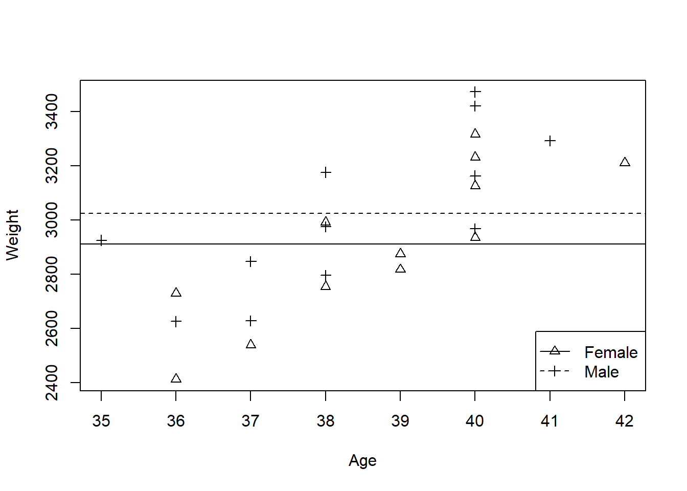
Figure 1.2: Predicted baby weights using a mean for each sex
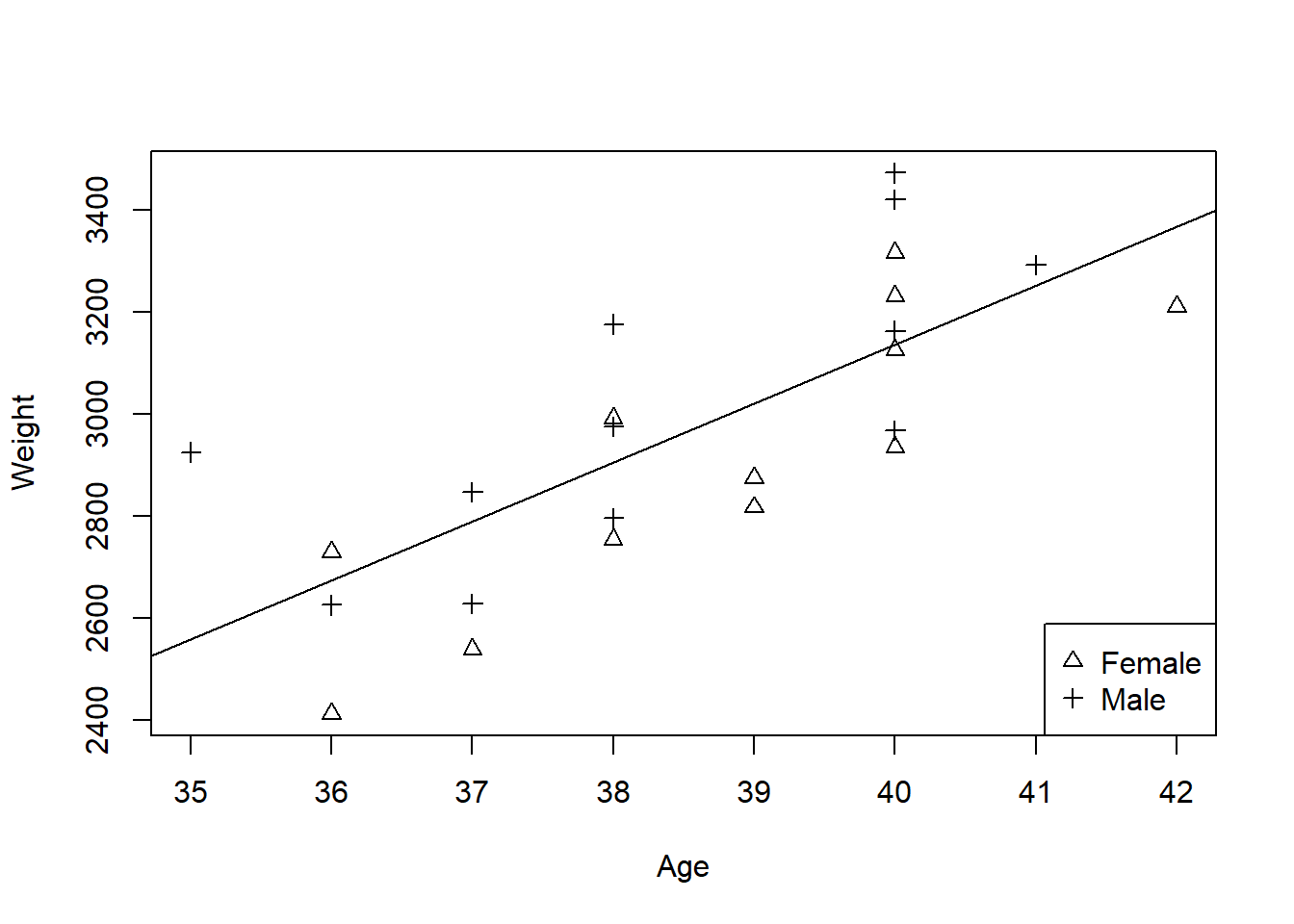
Figure 1.3: Predicted baby weights using age as a predictor
Figure 1.4 looks realistic. Both the differences between different ages and the differences between the sexes are accommodated.
Figure 1.5 permits the final possibility, that the lines are in fact of different slope. There is a slight tendency for female babies to increase in weight faster than males. This model is almost equivalent to fitting two regression lines separately to the male and female data, the only difference being that two separate models would fit two separate variances, one for each sex.
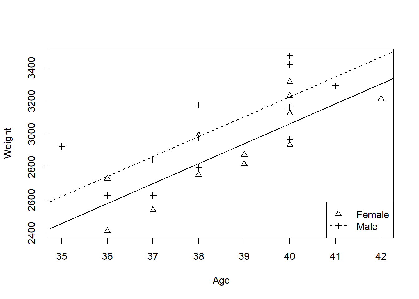
Figure 1.4: Predicted baby weights using a single slope but different intercepts for each sex
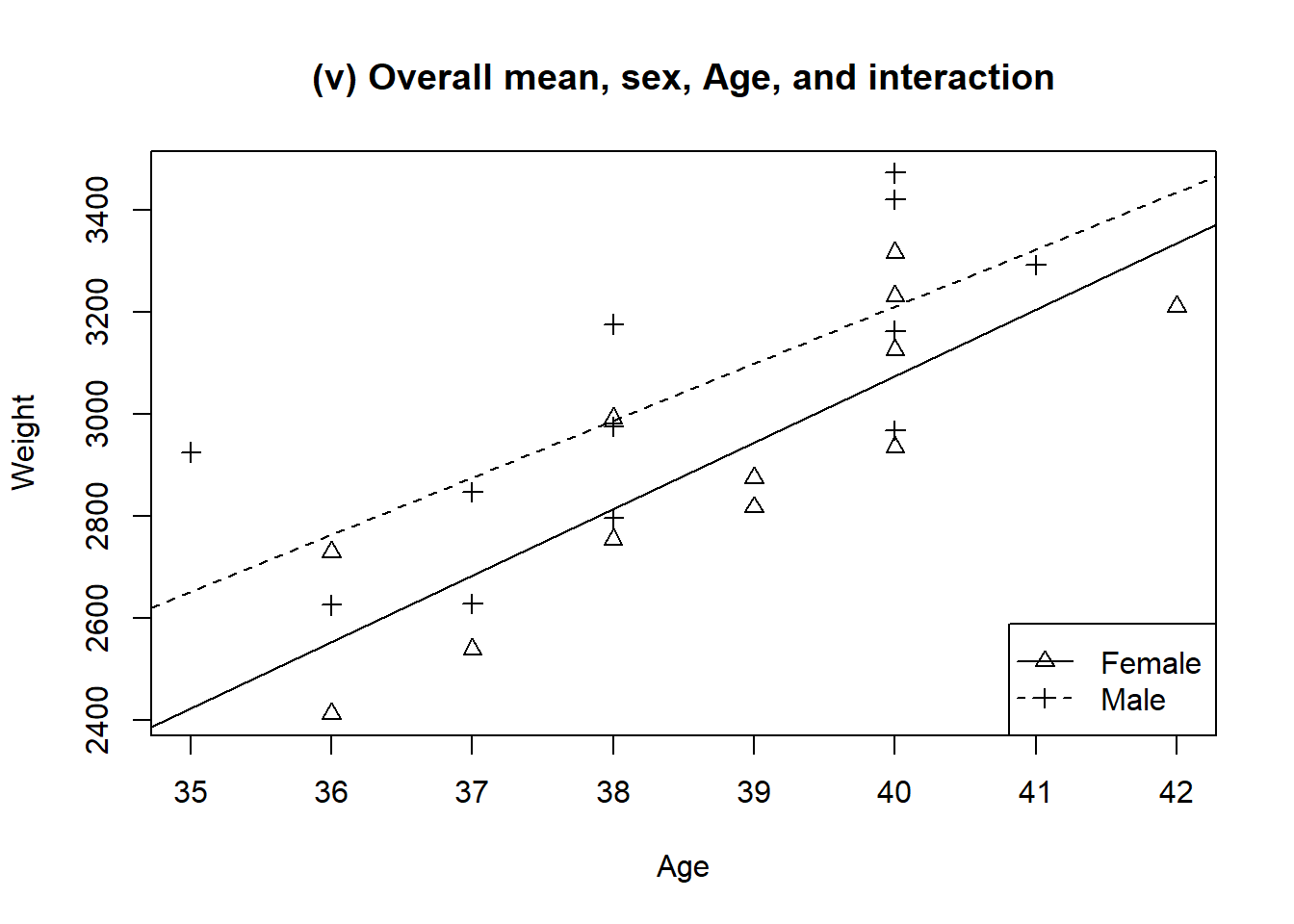
Figure 1.5: Predicted baby weights using different slopes and intercepts for each sex
Numerical discussion
Although a summary of a linear model usually takes the form of the equation of a line, in fact the ultimate use is a prediction. In this example a table giving the predicted weights of babies of both sexes at a range of gestational ages would be useful.
Table 1.2 shows fitted values for four ages for both sexes for all five models fitted thus far.
| Age | Gender | Model 1 | Model 2 | Model 3 | Model 4 | Model 5 |
|---|---|---|---|---|---|---|
| 36 | Female | 2968 | 2911 | 2674 | 2579 | 2553 |
| 38 | Female | 2968 | 2911 | 2905 | 2821 | 2814 |
| 40 | Female | 2968 | 2911 | 3136 | 3062 | 3074 |
| 42 | Female | 2968 | 2911 | 3367 | 3304 | 3335 |
| 36 | Male | 2968 | 3024 | 2674 | 2742 | 2763 |
| 38 | Male | 2968 | 3024 | 2905 | 2984 | 2987 |
| 40 | Male | 2968 | 3024 | 3136 | 3225 | 3211 |
| 42 | Male | 2968 | 3024 | 3367 | 3467 | 3435 |
The final column of Table 1.2 clearly shows that male and female babies grow at different rates. In other words there is an interaction between Age and Sex. To generate an informative table to reflect this model, (at least) four numbers are required: one male mean, one female mean, and the increases in weight for males and females. The other sets of fitted values require fewer numbers to illustrate the outcome.
The above descriptions spell out what should be obvious. In different situations different ways of describing the effects will be useful; note that a table will always be appropriate as long as we choose what to put in that table with careful reflection on what our modelling tells us.
The process above makes no distinction between categorical and quantitative variables. Describing the model, the table and the fitting process all involve just the names of the factors.
The word “general" in General Linear Model computer procedures means that categorical and quantitative variables can be handled together in this way. You will also come across Generalised Least Squares and Generalised Linear Models. These are quite different, and by the end of the course you will understand why.
Statistical discussion
Babies are variable. The numbers in Table 1.2 are estimates of mean values around which there is a great deal of variability. Do the small differences between columns of fitted values in Table 1.2 reflect true differences in the model, or just the variability between babies? Where should the refinement process mentioned in the previous section stop?
The standard statistical measure of goodness of fit is the residual sum of squares (RSS). The better the model, the smaller the RSS. A formal test statistic for the significance of any refinement is based on the resulting drop in residual sum of squares:
\[\begin{equation} F~ \mbox{statistic} = \frac{(\mbox{Drop in RSS})/(\mbox{df of drop})}{ (\mbox{RSS for maximal model})/(\mbox{df of maximal model})} \tag{1.1} \end{equation}\]
Figures 1.1 to 1.5 demonstrate this process for the baby weights example. The big drop in RSS is when age is added, and there is a smaller drop when sex is added. This is just what would be expected from the appearance of the graphs. The F value for the drop in RSS when the interaction is fitted is 0.19; it would have to be over 4.35 (\(F_{1,20; 0.05}\)) to be significant. The small differences between fitted values given in Table 1.2 could well reflect just the random differences between babies.
Algebraic discussion
All the preceding discussion has deliberately avoided explaining how the model \[Birthweight = Mean + Age + Sex + Age.Sex\] is translated into a regression model \[Y_i = \sum_{j=0}^k {\beta_j x_{ij}} = \boldsymbol{x}_i\boldsymbol{\beta}\] or \[\boldsymbol{Y} = \sum_{j=0}^k { \beta_j \boldsymbol{x}_j} = \boldsymbol{X}\boldsymbol{\beta}\] where \(\boldsymbol{x}_i\) is the (row) vector of explanatory variables for the ith case, \(\boldsymbol{\beta}\) is the (column) vector of regression coefficients, \(\boldsymbol{x}_j\) is the (column) vector of values for the jth explanatory variable, and \(\boldsymbol{X}\) is the “design" matrix with elements \(x_{ij}\).
Each computer program tackles the translation in its own way. However you may be familiar with the following, where ‘Sex’ is coded as a dummy variable:
Mean: \(\boldsymbol{x}_0\) is a column of 24 1’s, so \(\beta_0\) is the intercept.
Age: \(\boldsymbol{x}_1\) is age, so \(\beta_1\) is the increase in weight/week.
Gender: \(\boldsymbol{x}_2\) = 1 for males and 0 for females so \(\beta_2\) is (male weight - female weight).
You may not be so familiar with interaction terms. These can be represented by multiplying the columns for the single factors:
Age:GenderSex: \(x_{3i} = x_{1i}\times x_{2i}\) = 0 for females and \(age\) for males.
So \(\beta_3\) is (male weight gain/week - female weight gain/week).
An advantage of these definitions is that each \(\boldsymbol{x}\) column can be added in turn as the model is refined. If only the final model were of interest two lines would be fitted, one for males and one for females, which even the simplest software (including a pocket calculator) could handle. But there would then be no way of deleting a single column to test the interaction term for significance.
Having only two levels makes sex particularly easy to translate into \(\boldsymbol{x}\)’s. In general categorical variables require a set of \(\boldsymbol{x}\)’s, one fewer than the number of categories, and this whole set has to be added or deleted together. Nearly always the process will be invisible to us as users, but we will sometimes have to be careful when interpreting individual parameters.
1.3 Nested models
The birth weight example illustrates a sequence of nested models. Moving from Figure 1.1, to Figure 1.2 or 1.3, to Figure 1.4, and finally to Figure 1.5 the models includes the prior models as special cases. The F-test in Equation (1.1) only applies when comparing “nested" models. In this example, it corresponded to adding a parameter, but the minimum requirement for Model A to be nested in Model B is that if \(\boldsymbol{X}_{(A)}\) is the X-matrix for Model A and if \(\boldsymbol{X}_{(B)}\) is the X-matrix for Model B, any linear combination of the columns of \(\boldsymbol{X}_{(A)}\) must be able to be expressed as a linear combination of \(\boldsymbol{X}_{(B)}\).
This implies that for any fitted value using Model A \[\hat{y}_{(A)} = \boldsymbol{x} \boldsymbol{\beta}_{(A)}\] there will always be a \(\boldsymbol{\beta}\) giving the same fitted value using Model B, that is Model B can always fit as well as (and almost always better than) Model A. This will obviously be true if Model B is just Model A with extra columns.
To use the language of linear algebra, the space spanned by the rows of \(\boldsymbol{X}_{(A)}\) has to be a sub-space of the space spanned by the rows of \(\boldsymbol{X}_{(B)}\), so anything you can do with \(\boldsymbol{X}_{(A)}\) you can also do with \(\boldsymbol{X}_{(B)}\).
A familiar example is the goodness of fit test where each level of a single explanatory variable \(\boldsymbol{x}\) is replicated several times. Model 1 is then a regression model, (\(\boldsymbol{X}_{(A)}\) has a column of ones and a single column \(\boldsymbol{x}\)) and Model 2 is a one way anova model (\(\boldsymbol{X}_{(B)}\) has one column per level of \(\boldsymbol{x}\), each a dummy variable). The first column of \(\boldsymbol{X}_{(A)}\) is the sum of the columns of \(\boldsymbol{X}_{(B)}\) and the second column is the sum of the columns of \(\boldsymbol{X}_{(B)}\) after multiplying the ith row by \(x_{i}\). Each row of \(\boldsymbol{X}_{(A)}\) can thus be expressed as a linear combination of the columns of \(\boldsymbol{X}_{(B)}\) and so the regression model is nested in the ANOVA model.
In the next section we look at transformations. When \(\boldsymbol{X}_{(B)}\) is \(\log(\boldsymbol{X}_{(A))})\), Model B is not nested in Model A, or vice-versa. (Choose \(\boldsymbol{X} = (1, 2, 3, 4)^{T}\) and show that there is no way of finding a single \(\beta\) so that \((1, 2, 3, 4)^{T}\beta = \log(1, 2, 3, 4)^{T}\beta\).) An important consequence is that there is no test like the F-test in Equation (1.1) for assessing the value of a transformation.
1.4 Transformations
1.4.1 Example: Tree heights related to diameter.
This example is adapted from an exercise in (Bhattacharyya and Johnson 1977) (page 394). The data are given in Table 1.3, including some added columns for transformed variables.
| Diameter | Height | log Diameter | log Height |
|---|---|---|---|
| 0.9 | 18.0 | -0.1054 | 2.890 |
| 1.2 | 26.0 | 0.1823 | 3.258 |
| 2.9 | 32.0 | 1.0647 | 3.466 |
| 3.1 | 36.0 | 1.1314 | 3.583 |
| 3.3 | 44.5 | 1.1939 | 3.796 |
| 3.9 | 35.6 | 1.3610 | 3.572 |
| 4.3 | 40.5 | 1.4586 | 3.701 |
| 6.2 | 57.5 | 1.8245 | 4.052 |
| 9.6 | 67.3 | 2.2618 | 4.209 |
| 12.6 | 84.0 | 2.5337 | 4.431 |
| 16.1 | 67.0 | 2.7788 | 4.205 |
| 25.8 | 87.5 | 3.2504 | 4.472 |
Graphical discussion
Figures 1.6 , 1.7, and 1.8 show scatter plots for the data transformed in a variety of ways, with fitted lines for several models added. The second panel of these figures show plots of residuals for the model corresponding to the response and predictor variables used in the left panel of the figure. The raw data, Figure 1.6 suggests that a curve is probably more appropriate than a straight line, and that taking the logs of the Diameters will pull in the higher values, thereby straightening the line.
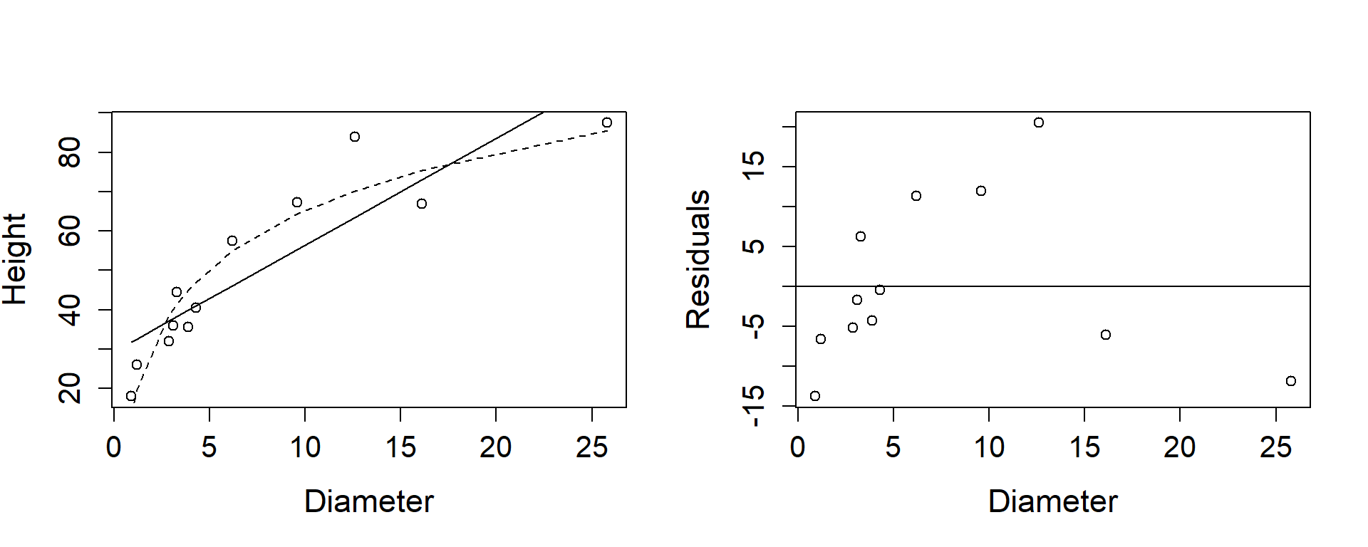
Figure 1.6: Tree heights and diameters, both on raw scale, with lines for fitted models added.
Figure 1.7 shows the result, a more plausible line. The residual plots emphasise the inadequacies in the fitted line, and whereas we might be happy with the height against log diameter plot, the residual plot perhaps suggests that the vertical spread of points around the line increases with increasing diameter. By plotting the log height against the log diameter the vertical spread is made to look even and a straight line quite satisfactory.
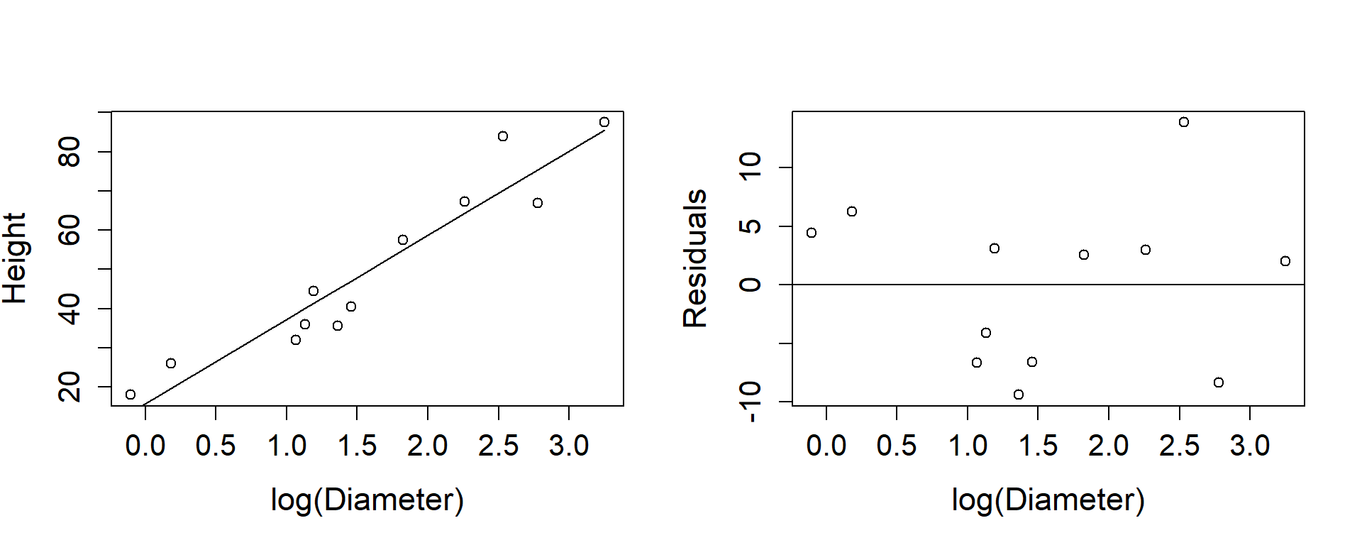
Figure 1.7: Tree heights and log of diameters
The horizontal spread is also uneven because there were more small trees than large ones. In the untransformed data the one large tree has considerable influence simply because it is out on its own. Indeed if the two right hand most trees had been higher a straight line might have seemed satisfactory and all discussion of transformations unnecessary. Taking the natural logarithm of the diameters spreads the points evenly along the axis, and makes the plot look better.
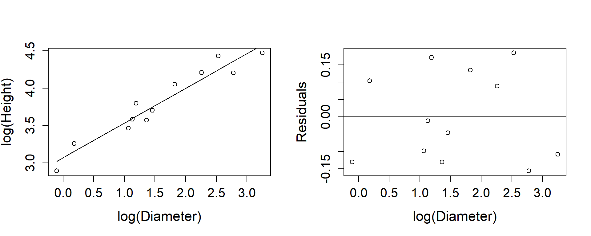
Figure 1.8: Tree heights and diameters both log-transformed.
Numerical discussion
The aim of this study is presumably to find a way of estimating the height of a tree from its diameter 4.5ft from the ground. Table 1.4 shows the estimate each model gives for trees of diameters 5, 10 and 25 inches.
| Mean | -SE | +SE | Mean | -SE | +SE | Mean | -SE | +SE | |
|---|---|---|---|---|---|---|---|---|---|
| 5 inch | 42.89 | 39.56 | 46.23 | 50.33 | 48.20 | 52.46 | 45.49 | 43.75 | 47.30 |
| 10 inch | 56.47 | 53.13 | 59.81 | 65.18 | 62.52 | 67.84 | 62.77 | 59.79 | 65.91 |
| 25 inch | 97.21 | 88.84 | 105.57 | 84.81 | 80.61 | 89.01 | 96.09 | 88.98 | 103.76 |
Obviously it does matter which model is fitted, particularly for the taller trees where there is little data. A statistician’s response to studies like these is invariably that the wrong data were collected, because without more wide trees no confident conclusions about the form of the model can be reached.
Statistical discussion
Hypothesis tests about the significance of the slope are really not relevant. Obviously height is related to diameter, and the important question is: how good is the prediction?
Table 1.4 has columns in it showing an interval obtained by using each regression model in turn, calculating
the standard error (SE) using the formula:
\[\begin{equation} \begin{aligned}
SD\left(\hat{y}\right) &=& \sqrt{Var(\hat{a}+\hat{b}x_0) + s^2}\\
&=&\sqrt{\left(\frac{1}{n} +
\frac{(x_0 - \bar{x})^2}{
S_{xx}}+1\right)\sigma^2}\end{aligned}
\end{equation}\]
\[\begin{equation}
SE\left(\hat{y}\right) = \sqrt{\left(\frac{1}{n} +
\frac{(x_0 - \bar{x})^2}{
S_{xx}}+1\right)s^2}
\tag{1.2}
\end{equation}\]
then calculating prediction + SE and prediction
– SE, back-transforming if necessary. You should plot these on the plot of
the untransformed data and note which looks most believable. Remember
that both your eye and the calculations are influenced by that one
widest tree.
If the points tend to lie on a curve but a straight line is fitted, the vertical distances of the points from the line will be larger than their distances from the curve. The points themselves do not change, just the curve through them, and if you measure the distances carefully you will find that the distances of the points from the line in Figure1.7 are the same as the distances from the corresponding curve in Figure 1.6. For these points \(s^2 = 54.3\) and for the untransformed data \(s^2 = 118.7\).
However when the response variable itself is transformed, as in Figure1.8, the distances of points from the fitted curve change. Moving up the curve points are pulled closer to the line, showing that transforming the response variable changes the variance structure as well as changing the form of the relationship between explanatory and response variable. Note that in Table 1.4, the differences between the + SE and – SE figures increases as the diameter increases.
Algebraic discussion
The actual form of the relationship is straight forward:
For model (i)
\[\begin{equation}
y = \alpha +\beta x
\tag{1.3}
\end{equation}\]
For model (ii)
\[\begin{equation}
\tag{1.4}
y = \alpha + \beta \log x
\end{equation}\]
which implies
\[\begin{equation} \begin{aligned}
\exp(y)&=& \exp\left(\alpha+\beta\log(x)\right)\\
&=& \exp(\alpha) x^\beta\\
&=& Ax^\beta,\quad\quad A=\exp(\alpha)\\\end{aligned}
\end{equation}\]
And for model (iii) \[\begin{equation} \tag{1.5} \log y =\alpha +\beta\log x \end{equation}\] which implies \[ y = Ax^\beta, \quad\quad A=\exp(\alpha)\]
A physicist may well be able to choose between these models for us, although a living structure like a tree is much more difficult to analyse than a rod or a pipe. From quite crude considerations, like the height of a zero width tree, Equations (1.3) and (1.4) seem implausible. At least Equation (1.5) does predict that diameter and height tend to zero together. If you look again at Figure 1.7 you will see that the predicted heights of the two smallest trees are too low, which is what might be expected from an equation which predicts that ultimately heights become negative.
1.5 Giving points different weights
1.5.1 Example: Age and jaw length of deer.
(Brook and Arnold 1985) (page 87) give data from 712 male deer shot in the Ruahine ranges, relating the jaw length of the deer to its age. The data are reproduced in Table (tab:DeerJawData) and plotted in Figure 1.9.
| Age | Midage | Number | JawLength | SD |
|---|---|---|---|---|
| <1 | 0.5 | 71 | 185.9 | 21.24 |
| 1+ | 1.5 | 250 | 231.8 | 16.64 |
| 2+ | 2.5 | 210 | 254.8 | 15.30 |
| 3+ | 3.5 | 59 | 272.5 | 11.08 |
| 4+ | 4.5 | 44 | 271.5 | 12.93 |
| 5+ | 5.5 | 34 | 278.3 | 10.03 |
| 6+ | 6.5 | 12 | 284.9 | 7.24 |
| 7+ | 7.5 | 9 | 281.8 | 11.05 |
| 8+ | 8.5 | 8 | 285.0 | 13.30 |
| 9+ | 9.5 | 7 | 272.3 | 17.73 |
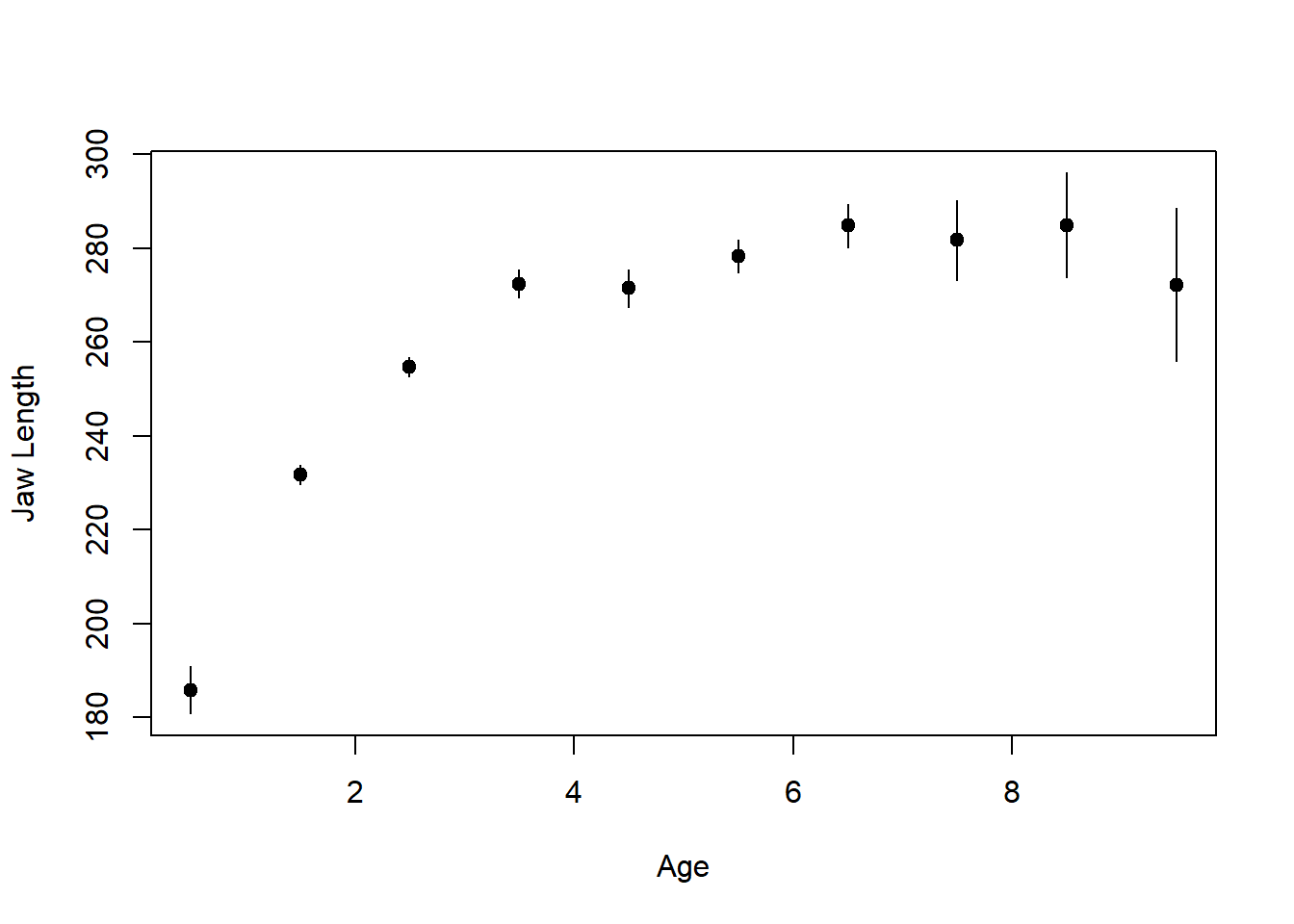
Figure 1.9: Plot of summarised deer jaw data.
Graphical discussion
Clearly some transformation is required for this data. (Brook and Arnold 1985) fit jaw length to the log of age, as shown in Figure 1.10 and this fits moderately well.
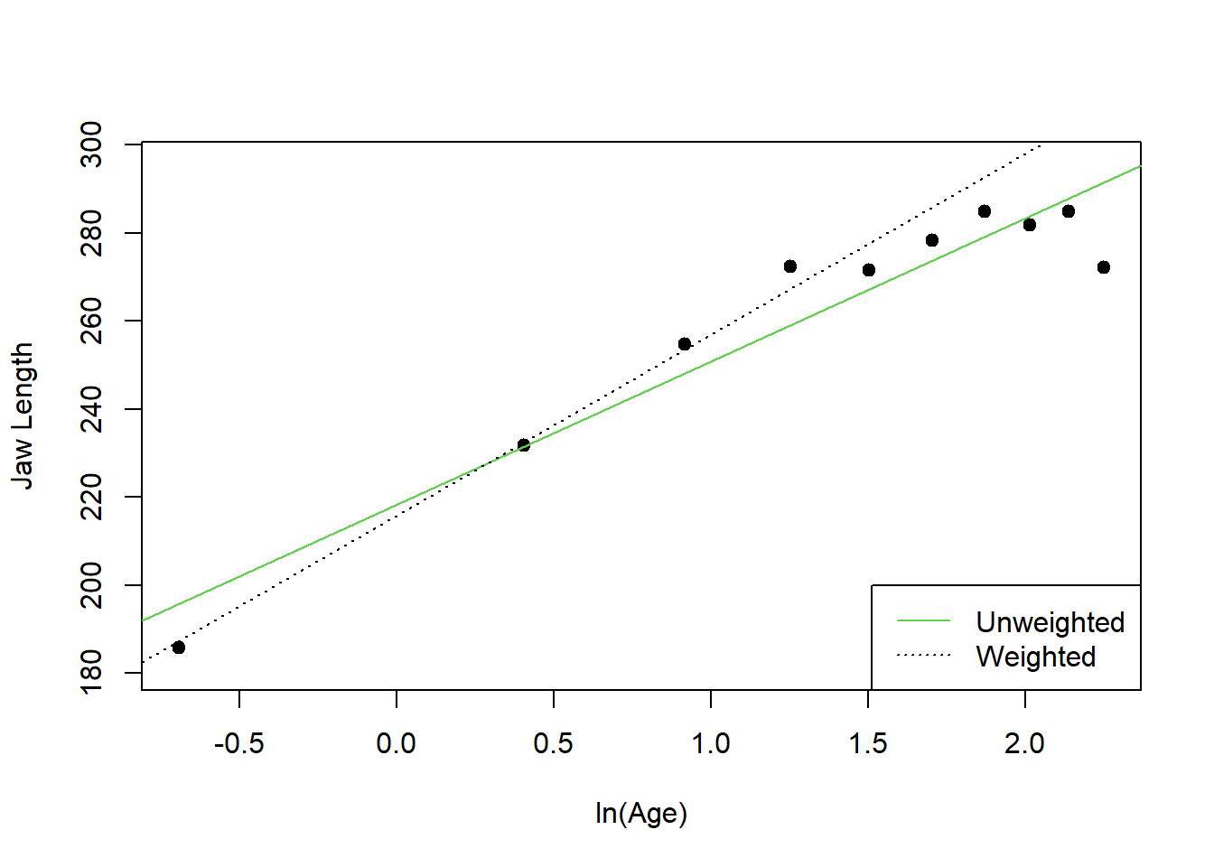
Figure 1.10: Model fitted to the deer jaw data by Brook and Arnold (1985)
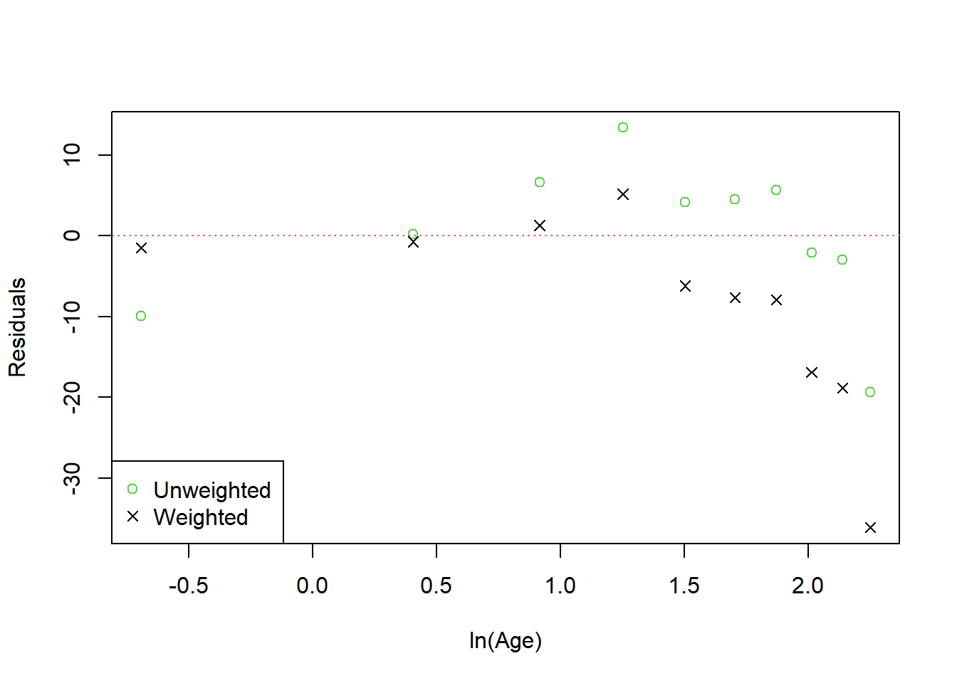
Figure 1.11: Residuals for the weighted and unweighted regression models fitted to the Deer Jaw data.
However the accompanying residual plot suggests that there is still curvature. Experience suggests that growth stops when it reaches a maximum, and the figures suggest that after about 6 years jaw lengths stop increasing. What is needed is a curve which approaches a maximum figure asymptotically. Just what this curve might be is discussed in the mathematical discussion below.
Another difference between this and the preceding example is that each point is the mean of many deer. The standard deviations of the age groups given in Table 1.5, shows that young animals have more variable jaw lengths than middle-aged ones. There is some evidence that variability increases in old animals, but because sample sizes are small the estimates of variability are themselves variable.
The lines in Figure 1.9 show a 95% confidence interval for each mean. Because the numbers vary greatly between the different age groups the precision of each point also varies greatly, and this should be taken into account when the model is fitted. For example, in the model proposed by (Brook and Arnold 1985), the deer of age 0.5 years are on their own well out to the left and are clearly very influential. Note however, their jaw lengths have a large standard deviation and there are only a third as many of them as in each of the next two age categories. Furthermore, there are only 36 deer altogether 6+ or older, only two more than are in the single 5+ category. These four categories together should be given about the same weight as the single 5+ category. If points are weighted according to the standard error of their mean the result is the dotted line in Figure 1.10. Note how much worse this line fits the older deer though.
Mathematical discussion
What is the equation of a curve which rises to an asymptote? There are
many, but a commonly used one is
\[\begin{equation}
y = A - B e^{-kt}
\tag{1.6}
\end{equation}\]
As t becomes large the \(Be^{-kt}\) term tends
to zero and y tends to A. Unfortunately this curve cannot be written
as a linear model. As written y is a linear function of \(e^{-kt}\), but
\(e^{-kt}\) cannot be calculated without knowing k. Some rearrangement
gives \[A - y = B e^{-kt}\] or
\[\begin{equation}
\log(A-y)= \log B - kt
\tag{1.7}
\end{equation}\]
which expresses \(\log(A -y)\) as a linear
function of t, but \(\log(A -y)\) cannot be calculated without knowing
A. We have here an example of a non linear model, and it is included
here as an example of what we are not going to learn about. However, in
fact this particular model is reasonably easy to fit and the process
will be outlined in the computational discussion. There is a
mathematical complication however.
Figure 1.9 suggests that a reasonable guess for A might
be 285 as this is the mean jaw length for the 8+ age group. On the other
hand, a few individual deer have jaw lengths greater than this.
Given a value for A, \(\log B\) and k can be found as explained previously. The complication is that logs are only defined for positive quantities, and a guess of A = 285 means that \(A-y\) will be negative for some individual deer. Equation (1.7) is therefore not a suitable form for fitting stochastic data.
Statistical discussion
To follow the final sentence of the mathematical discussion, the observed random Y varies from the mean \(\mu_Y\), and although \(A-\mu_Y\) is always positive, \(A-Y\) might not be. Equations (1.6) and (1.7) may be equivalent mathematically, but they imply different probability distributions for Y. The standard assumptions about distributions in linear regression add the following to the model:
For Equation (1.6): Y has a normal distribution with constant variance.
For Equation (1.7): \(\log(A- y)\) has a normal distribution with constant variance.
In this example though, the variance of Y, the jaw length, is not constant. The data shows that the standard deviation decreases from about 20 for babies to about 10 for mature animals. This conflicts with the model of Equation (1.6).
If \(\log(A -y)\) has constant variance \(\sigma^2\), \((A - y)\) has variance proportional to \(\sigma^2(A -\mu_Y)^2\). (This will be proved in Chapter 2. As animals become older \(\mu_Y\) becomes very close to A and so the variance of y must become vanishingly small, but for baby animals \(\mu_Y\approx\) 190 and the variance of y is \(\sigma^2 \times90^2\). This grossly overstates the change in variance, and the model in Equation (1.7) is therefore much worse than the one in Equation (1.6).
There are two separate topics involved here: transformations, and weighting points depending on their variance. The theory of these will be explained in Chapter 2, so some empirical observations will suffice here. The same weighted regression which can accommodate different numbers in each group can also accommodate different variances.
Figure 1.10 shows the unweighted regression line compared with the line fitted with each point weighted in this way. However the ideal would be to have the variance of each point incorporated in the model directly rather than requiring a separate empirical estimate at each point. An important component of this course is to use weighted regression to fit a model where the variance of y varies depending on x, but where the data does not provide a direct estimate of it.
Computational discussion
There are two complications with this example. Firstly, how can points be weighted differently, and secondly how is k estimated in the \(e^{-kt}\) term?
The theory of weighted least squares will be revised in Chapter 3. The principle is simple enough though. The
variance of the mean of n observations is \(\sigma^2/n\), so if we want
a point to have variance \(\sigma^2/w_i\), that is, to have weight \(w_i\)
(the less the variance the greater the weight), we are in effect,
treating it as if it were \(w_i\) identical observations. For example if
the sum of squares for n independent observations (which are equally
weighted) is \(S_x\): \[S_x= \sum_{i=1}^n {(x_i-\bar{x})^2}\]becomes
\[\begin{equation}
(\#eq:WeightedS_x)
S_x= \sum_{i=1}^n {w_i(x_i -\bar{x})^2}
\end{equation}\]
and similarly for all the
other sums of squares and cross product formulas. This is just the same
as the grouped data formula, except that the \(w_i\) need not be an
integer. Note that the degrees of freedom are not affected. Only a
genuinely different observation contributes a degree of freedom.
There is no direct linear regression formula to estimate k. The goal is to minimise the variance of predictions of the response variable y, and this is done by minimising the residual sum of squares. There are several ways of doing this, and all amount to refined trial and error. Much of our work in this course will require minimisation of residual sums of squares, so a description of the process follows even though in practice it will happen inside a computer. As an aside, there is a nonlinear regression function that can do all of this, but we need to illustrate a point here.
Find a good initial value.
Fitting A = 285.01 in the model of Equation (1.7) gives \(k_0= 0.634\)
Fit the model of Equation (1.6) with this \(k_0\), then another value that is a little greater than \(k_0\), and a value a little lower than \(k_0\), and find the corresponding residual sums of squares:
Setting k = 0.534, 0.634, 0.734 gives RSS = 237, 159, 166 respectively.
Plot the three points on a graph of residual sums of squares against k, and draw a smooth curve through them (see Figure 1.12.
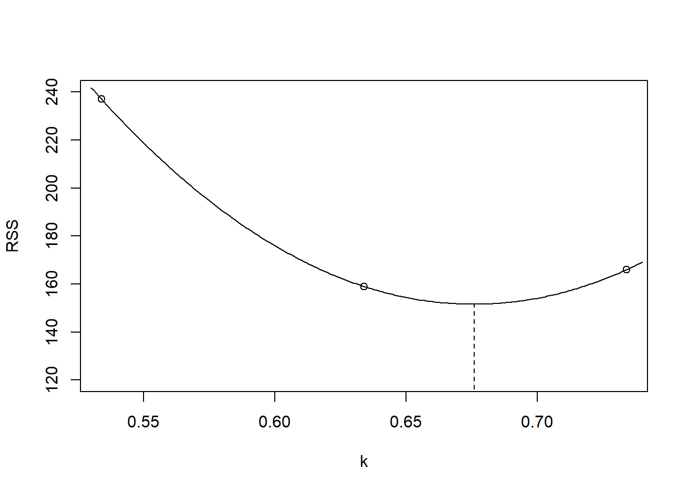
Figure 1.12: Finding the optimal value for k.
- Choose the minimum of this curve as the best guess for k. This best guess could be used as a new initial value and the process repeated, but the curve is quite flat so further iteration will not decrease the residual sum of squares by a worthwhile amount.
1.6 Summary
A number of topics have been discussed informally:
The starting point for a model is a response variable and (possibly several) explanatory variables.
General Linear Model procedures enable categorical variables to be incorporated in a model in the same way as quantitative variables.
Finding a ‘good’ model is a process of refinement, starting with main effects, then adding their interactions, using an F-test (for nested models) and residual plots to assess each stage.
There are two components to a model:
- The relationship between the mean of the response variable \(\mu_Y\) and the explanatory variables.
- The (conditional) distribution, and in particular the variability of the response variable.
In a conventional linear model \[\begin{equation} \mu_{Y_i} = \sum{\beta_j x_{ij}} = \boldsymbol{\beta}^T \boldsymbol{x}_i \end{equation}\]
and \(\mu_Y\) has a normal distribution, \(\sigma_{Y_i}^2\) is constantTransformations can convert a number of problems into the conventional frame work, but not all of them. Messy iterative procedures are then needed.
Our future work will centre on generalising point 5.
1.7 Exercises
- Use R to calculate separate regression lines for the male and female babies in Example 1.2.1, and derive the parameters in Figures 1.1 to 1.5.
This exercise is used as an in-class tutorial.
- Using the data on the heights and diameters of trees, calculate a regression of height on diameter and height on \(\log(\mbox{Diameter})\) omitting the largest tree in Example 1.4.1. Replot Figures
- and (ii). Which of the two regressions would you choose, and why?