Chapter5 Binary Logistic Regression
Chapter Aim: You will have met logistic regression models earlier, but the aim here is to show how it fits into the generalised linear models framework.
5.1 What is logistic regression?
Logistic regression is used when the response is just success or failure. Typical examples are where success = death (for an insecticide) or cure (for a drug). The data for mortality of beetles (Example 2.4.1) is an example of the former case. More generally logistic regression can be used for any data where the response is either In or Not in a category. Such data are called binary data. Each observation is a zero or a one, and its expected value is \(\pi\), the probability of a one. It is this probability which the generalised linear model predicts.
Very often a group of observations are made under the same conditions, so that \(\pi\) is the same value. The total number of successes in the group is then a binomial random variable. Logistic regression is also used to model this binomial data.
5.2 An alternative to the chi-square test
5.2.1 Example: A drug trial
This example is taken from (McCullagh and Nelder 1989), and refers to a study of the effect of the drug sulphinpyrazone on cardiac death after myocardial infarction. A total of 1475 people were split into two groups, one group being given the drug, the other the placebo. Table 5.1 gives the number of deaths from all causes at the end of the trial period.
| Deaths (all causes) | Survivors | Total | |
|---|---|---|---|
| Sulphinpyrazone | 41 | 692 | 733 |
| Placebo | 60 | 682 | 742 |
| Total | 101 | 1374 | 1475 |
(Deaths from all causes are recorded in case side effects of the drug increase the chance of deaths from causes unrelated to myocardial infarction.)
You will recognise this as a simple comparison of two proportions for which a chi-square test could be used. The subscripts P and S are used to identify the two groups.
To formulate it as a GLM put:
\(\boldsymbol{\beta}^T\boldsymbol{x}\) \(=\beta_0\) for placebo. \(= \beta_0 + \beta_1\) for drug. \(Y_P / n_P\) = proportion of deaths in placebo group \(Y_S / n_S\) = proportion of deaths in treated group \(Y_i\) has a binomial distribution, \(B(n_i , p_i)\), \(i = P\) or S.
\(E(Y_i) = p_i.\) With only two points \(g(\mu)\), the link function, could be anything, so it can be taken to be the identity. Later we will see that there are reasons to make it more complicated.
Likelihood
\(\beta_0\) is the probability that an individual given the placebo dies. From the binomial distribution, the probability that 60 of the 742 placebo patients die is \[f_P(60) = \left( \begin{array}{c} 742 \\ 60 \end{array} \right) \beta^{60}_0 (1 - \beta_0)^{682}\]
\(\beta_0 + \beta_1\) is the probability that an individual given the drug dies. Again from the binomial distribution, the probability that 41 of the 733 die is
\[f_S(41) = \left( \begin{array}{c} 733 \\ 41 \end{array} \right) (\beta_0 + \beta_1)^{41}(1 - \beta_0 - \beta_1)^{692}\]
Maximum likelihood finds the values of \(\beta_0\) and \(\beta_1\) which maximise the probability of both these events.
\[L(\beta_0 , \beta_1) = \left( \begin{array}{c} 733 \\ 41 \end{array} \right) (\beta_0 + \beta_1)^{41}(1 - \beta_0 - \beta_1)^{692} \left( \begin{array}{c} 742 \\ 60 \end{array} \right) \beta^{60}_0 (1 - \beta_0)^{682}\] %(5.3)
Since sums are easier to work with than products, form \(\ell=\ln(L)\): \[\begin{equation} \ell(\beta_0 , \beta_1 ) = k + 41 \ln(\beta_0 + \beta_1 ) + 692 \ln(1 - \beta_0 - \beta_1 ) + 60 \ln \beta_0 + 682 \ln(1 - \beta_0 ) \tag{5.1} \end{equation}\]
The binomial coefficients are constant and do not affect comparisons. If the drug has no effect \(\beta_1 = 0\), and the likelihood is
\[\begin{equation} \ell(\beta_0) = k + 41 \ln \beta_0 + 692 \ln(1 - \beta_0 ) + 60 \ln \beta_0 + 682 \ln(1 - \beta_0) \tag{5.2} \end{equation}\]
Now, the maximum likelihood estimate of the binomial p is just the sample proportion. So we substitute \(\frac{60}{742}\) for \(\beta_0\) and \(\frac{41}{733}\) for \((\beta_0 + \beta_1)\) in Equation (5.1) and the combined proportion \(\frac{101}{1475}\) for \(\beta_0\) in Equation (5.2). If there is a difference between drug and placebo the maximum value of \(\ell\) is therefore \[k + 41 \ln \frac{41}{733} + 692 \ln \frac{692}{733} + 60 \ln \frac{60}{742} + 682 \ln \frac{682}{742} = k - 366.464\]
If there is no difference between drug and placebo the maximum value of \(\ln L\) is a little smaller: \[k + 101 \ln \frac{101}{1475} + 1374 \ln \frac{1374}{1475} = k - 368.271\]
and the difference, \(368.271 - 366.464 = 1.807\), results from one parameter \(\beta_1\). From the theory in Chapter 4, \(2 \times\) (drop in \(log\) likelihood) has a \(\chi^{2}_{1}\) distribution. Its value is \(2 \times 1.807 = 3.61\). Compared with \(\chi^{2}_{1, 0.95} = 3.84\) this has a P-value a little larger than 5%, suggestive of a treatment effect but hardly conclusive.
The standard \(\chi^2\) test gives a value 3.59, very close to the likelihood ratio statistic, but not exactly the same. With smaller samples the difference can be larger.
The Link Function
With just two points it may seem unnecessary to even consider a link function. The question is, what is the most useful statistic for measuring the difference resulting from the use of the drug? \(\beta_1\), used above, is equivalent to \(p_1 - p_2\), which is simple and easy to understand. The variance of \(\hat{p}_1 - \hat{p}_2\) ranges from \(\frac{1}{2n}\) when \(p_1\) and \(p_2\) are around 0.5 to approaching zero when \(p_1\) and \(p_2\) are around zero or one. The difference between 0.10 and 0.05 may be important, but that between 0.50 and 0.45 not. Intuitively a difference between 0.05 and 0.10 seems more significant in an every day sense, too. After all it corresponds to a doubling.
An alternative statistic is the odds ratio. Punters will be familiar with odds, which equal the ratio \(p:(1- p)\). Even odds or 1:1 (= 1) imply p = 0.5, 2:1 (= 2) implies \(p = 2/3\), 100:1 (= 100) implies \(p = 100/101\) and 1:100 (= 0.01) implies \(p = 1/101\).
| \(p_1\) | \(p_2\) | Odds ratio | \(log\)(Odds) |
|---|---|---|---|
| 0.1 | 0.05 | (0.1/0.9)/(0.05/0.95) = 2.11 | 0.747 |
| 0.2 | 0.1 | (0.2/0.8)/(0.1/0.9) = 2.25 | 0.811 |
| 0.5 | 0.45 | (0.5/0.5)/(0.45/0.55) = 1.22 | 0.201 |
| 0.65 | 0.6 | (0.65/0.35)/(0.6/0.4) = 1.24 | 0.214 |
| 0.9 | 0.95 | (0.9/0.1)/(0.95/0.05) = 0.474 | -0.747 |
The odds ratio compares two odds by their ratio. Some examples of odds ratios are given in Table 5.2. The ratio tends to work like a multiplicative scale for values of p near 0 or 1 (the log odds ratio is much the same whether doubling from 0.05 to 0.1 or from 0.1 to 0.2), and like an additive scale for p values near 0.5 (the log odds ratio is much the same whether 0.05 is added to 0.5 or 0.6).
These are the values which are going to be put equal to a linear function of the x’s, so logs must be used to ensure that reversing \(p_1\) and \(p_2\) merely reverses the sign of \(\boldsymbol{\beta}^T\). It also avoids problems with negative values of \(\boldsymbol{\beta}^T \boldsymbol{x}\) since the log odds ratio can range over the entire number line.
We have constructed the logit transformation:
\[\begin{equation} \boldsymbol{\beta}^T \boldsymbol{x} = \eta = logit(p) = log \frac{p}{1 - p} \tag{5.3} \end{equation}\]
which can be inverted: \[\begin{equation} p = \frac{e^{\eta}}{1 + e^{\eta}} \tag{5.4} \end{equation}\]
The logit transformation has an interesting property which makes it valuable for studying the effects of exposure to a possibly harmful pollutant. Either separate samples can be taken from the exposed group and non exposed, called a prospective study, or separate samples can be taken from those who are diseased and not diseased, called a retrospective study.
| Diseased | Healthy | Total | |
|---|---|---|---|
| Exposed | \(p_{00}\) | \(p_{01}\) | \(p_{0.}\) |
| Not Exposed | \(p_{10}\) | \(p_{11}\) | \(p_{1.}\) |
| Total | \(p_{.0}\) | \(p_{.1}\) | 1.0 |
In a prospective study (looking forward) an exposed group is compared with a group which was not exposed, and the odds of being diseased are estimated separately for the two groups. The estimates are \(p_{00} / p_{01}\) and \(p_{10} / p_{11}\) respectively, so the log ratio is \[\ln\left(\frac{p_{00}}{p_{01}}\right) - \ln\left(\frac{p_{10}}{p_{11}}\right) = \ln\left( \frac{p_{00}p_{11}}{p_{10}p_{01}}\right)\]
In a retrospective study (looking back) a diseased group is compared with a healthy group, and the odds of being exposed are estimated separately for these groups. The estimates are \(p_{00}/ p_{10}\) and \(p_{01}/ p_{11}\) respectively, so the log ratio is \[\ log\left(\frac{p_{00}}{p_{10}}\right) - \ln\left(\frac{p_{01}}{p_{11}}\right) = \ln \left(\frac{p_{00}p_{11}}{p_{10}p_{01}}\right),\] the same log odds ratio. Other forms of estimates give different values for these two situations.
Fitted values of 0 or 1 will clearly cause problems for the logit (and other) link functions. However fitted values of 0 or 1 are rare. On the other hand data values of 0 or 1 are common. For this reason the starting values for iterations cannot just be y. Instead use \[\hat{\mu}_0 = (n_{i} y_{i} + 0.5)/( n_{i} + 1)\]
5.3 Dose response models
A common problem is finding the relationship between the dose of a drug and the probability of cure. Again, the statistical problem is the same as finding the relationship between the dose of a pesticide and the probability of death. Underlying the dose response model is the idea that tolerance to a drug varies over the population according to a distribution called the tolerance distribution, \(h(s)\). The proportion killed by a dose \(s_0\) is then \(\int_{-\infty}^{s_0} h(s) ds\). This integral is a function of the dose, and satisfies all the requirements of a link function. Indeed the very first commonly used extension of a generalised linear model was probit analysis, which is a dose response model where the tolerance distribution is the normal distribution. This is a generalised linear model where Y has binomial distribution and \[E(Y) = p = \Phi(\boldsymbol{\beta}^T \boldsymbol{x})\] \(\Phi{}\) being the cumulative normal distribution function.
5.3.1 Example: Mortality of beetles (Example 2.4.1 revisited)
In the previous analysis of this data the angular transformation was used to allow for the variance changing as the mean changed. Recall that the main problem for this transformation approach was that the prediction intervals for fitted values near one were flawed. Using a generalised linear model we can find the maximum likelihood estimate for a binomial distribution and independently seek the best fitting link function. The probit and logit link functions are quite similar, both being symmetric S-shaped curves. An alternative is the complementary log-log function (aka Extreme value) arising from the rather skew tolerance distribution \(h(s) = \beta_2 exp[(\beta_1 + \beta_2 s) - exp(\beta_1 + \beta_2 s)]\). Integrating this gives the link function \(\ln[-\ln(1 - p)]\). Table 5.4 shows the results of fitting these to the beetle data.
    data(Beetles, package="ELMER")
Beetles = Beetles |> mutate(NoLiving = NoBeetles - NoKilled)
    # with logit function
    Model = glm(cbind(NoKilled,NoLiving)~Dose,data=Beetles,family=binomial(link="logit"))
    # or
    Model = glm((NoKilled/NoBeetles)~Dose,data=Beetles,family=binomial(link="logit"),weights=NoBeetles)
    Beetles$fit.Logit = round(fitted(Model)*Beetles$NoBeetles,2)

    # with probit function
    Model.probit = glm(cbind(NoKilled,NoLiving)~Dose,data=Beetles,family=binomial(link="probit"))
    Beetles$fit.Probit = round(fitted(Model.probit)*Beetles$NoBeetles,2)

    # with extreme value fitted values
    Model.extreme = glm(cbind(NoKilled,NoLiving)~Dose,data=Beetles,family=binomial(link="cloglog"))
    Beetles$fit.ExtremeValue = round(fitted(Model.extreme)*Beetles$NoBeetles,2)
#Beetles| log10 Dose | Number Treated | Number Killed | Fitted Logistic | Fitted Probit | Fitted Extreme Value |
|---|---|---|---|---|---|
| 1.691 | 59 | 6 | 3.46 | 3.36 | 5.59 |
| 1.724 | 60 | 13 | 9.84 | 10.72 | 11.28 |
| 1.755 | 62 | 18 | 22.45 | 23.48 | 20.95 |
| 1.784 | 56 | 28 | 33.90 | 33.82 | 30.37 |
| 1.811 | 63 | 52 | 50.10 | 49.62 | 47.78 |
| 1.837 | 59 | 53 | 53.29 | 53.32 | 54.14 |
| 1.861 | 62 | 61 | 59.22 | 59.66 | 61.11 |
| 1.884 | 60 | 60 | 58.74 | 59.23 | 59.95 |
| Logistic | Probit | Extreme Value | |
|---|---|---|---|
| Beta0 | -60.72 | -34.94 | -39.57 |
| Beta1 | 34.27 | 19.73 | 22.04 |
| Deviance | 11.23 | 10.12 | 3.45 |
The deviance statistic with 8 points fitted and 2 parameters estimated will approximate a \(\chi^{2}_{6}\) distribution, the 95% point of which being 12.59. Both the probit and logit models are very close to this, but the extreme value model gives a much smaller value, indicating a better fit.
An important assumption of the binomial distribution is that each beetle was killed independently. More likely a number of beetles would have been sprayed as a group, perhaps as 6 groups of 10, raising the practical possibility that each group had a different \(\pi\). This could be an explanation for the deviance being a little high. Before accepting the extreme value model we would have to find out exactly how the experiment was performed.
5.4 Binary data
In the preceding examples the response was a binomial random variable \(B(n,\pi)\) with n reasonably large. The great advantage of using logistic models though is that there can be continuous covariates which are unique for every observation. The \(y_{i}\) are then either 0 or 1, and these can be fitted to quantitative explanatory variables that have different values for each individual, estimating a unique \(\pi_{i}\) for each.
It makes no essential difference to the likelihood function whether a binomial random variable is counted as X successes in n trials, or as n independent observations of which X are successes.
In the first case the likelihood is \[L(\pi) = \left( \begin{array}{c} n \\ x \end{array} \right) \pi^x (1- \pi)^{n-x}\] and in the second it is \[L(\pi) = \pi^x (1 - \pi)^{n-x}\]
As we saw in Section 5.2 the term \(\left( \begin{array}{c} n \\ x \end{array} \right)\) is a constant which does not affect the maximum or the shape of the likelihood function.
The inferences however are only true asymptotically, that is for large n. Although the total sample will usually be large, a binomial parameter of only 1 is so far from ‘large’ that the size of the deviance has little relationship to the goodness of fit. Changes in deviance between different models may however still be used to compare models. They may be compared with a \(\chi^{2}\) distribution or compared with the dispersion using an F-test. The latter is a more robust test.
5.4.1 Example: Spinal surgery data
This example was quoted by (Chambers and Hastie 1992). The measurements come from 81 children following corrective spinal surgery. The binary outcome variable is presence or absence of a post operative deformity called Kyphosis. Explanatory variables are Age, the age of the child in months, Number, the number of vertebrae involved in the operation, and Start, the beginning of the range of vertebrae involved. Boxplots summarising the data are shown in Figure 5.1. The presence of Kyphosis appears to be associated with older children, more levels, and lower start levels. The output below Figure 5.1 shows the result of fitting a GLM with a logit link function. Absence of Kyphosis is coded as 0.
    data(Kyphosis, package="ELMER")
    par(mfrow=c(1,3))
    plot(Age~Kyphosis, data=Kyphosis)
    plot(Kyphosis$Kyphosis, Kyphosis$Number, xlab="Kyphosis", ylab="Number")
    plot(Kyphosis$Kyphosis, Kyphosis$Start, xlab="Kyphosis", ylab="Start")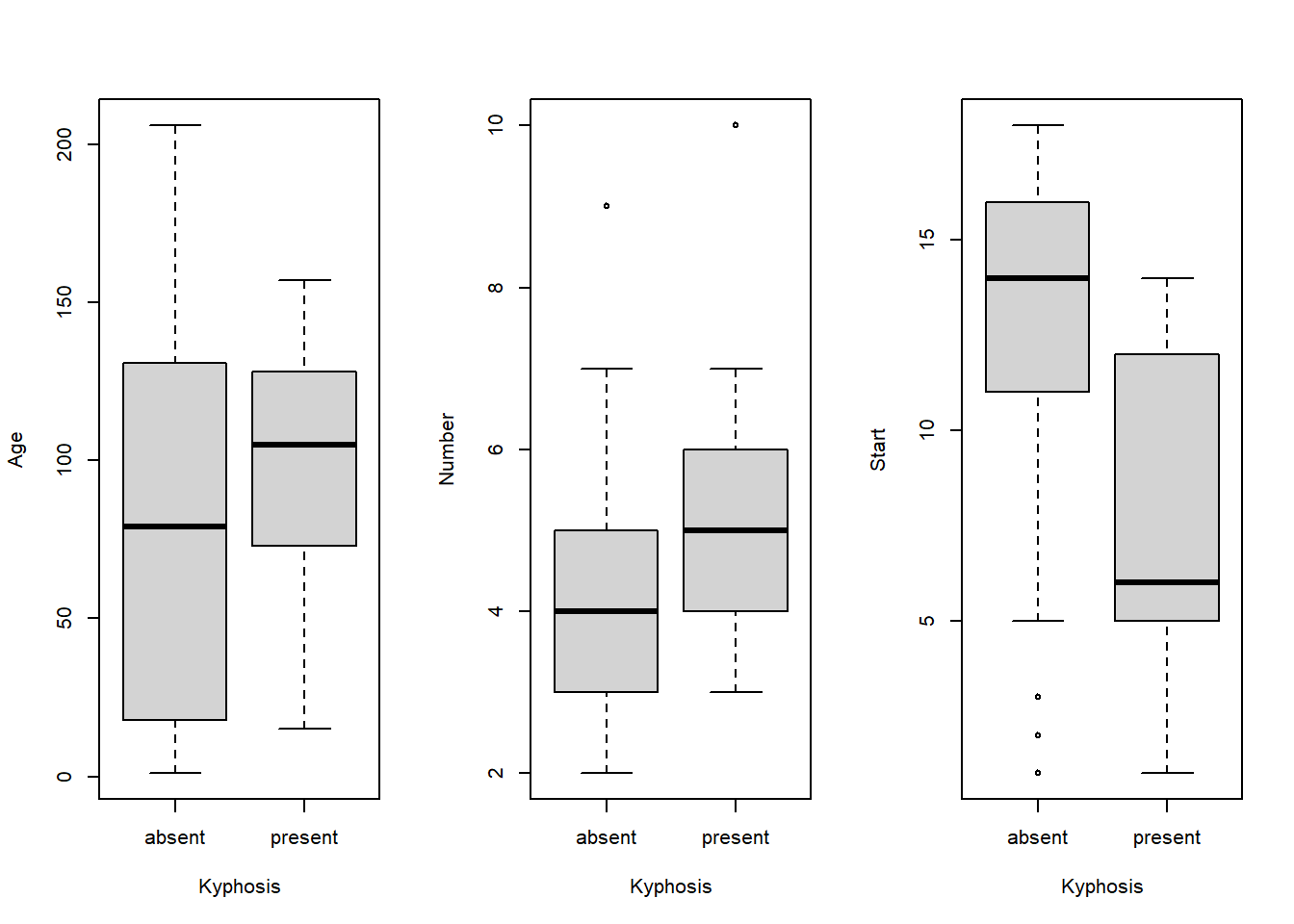
Figure 5.1: Boxplots for Kyphosis data
Call:
glm(formula = Kyphosis ~ Age + Number + Start, family = binomial,
    data = Kyphosis)

Coefficients:
            Estimate Std. Error z value Pr(>|z|)
(Intercept) -2.03693    1.44957   -1.41   0.1600
Age          0.01093    0.00645    1.70   0.0900 .
Number       0.41060    0.22486    1.83   0.0678 .
Start       -0.20651    0.06770   -3.05   0.0023 **
---
Signif. codes:  0 '***' 0.001 '**' 0.01 '*' 0.05 '.' 0.1 ' ' 1

(Dispersion parameter for binomial family taken to be 1)

    Null deviance: 83.234  on 80  degrees of freedom
Residual deviance: 61.380  on 77  degrees of freedom
AIC: 69.38

Number of Fisher Scoring iterations: 5
The t values (which can be very approximate with binary data) suggest that Start is an important explanatory variable and that Age and Number cannot be ignored. Their signs are just as the boxplots would suggest. For example, each extra month of age increases the log odds of presence of Kyphosis by 0.01. The drop in deviance from 83.23 to 61.38 (21.85) is highly significant.
As with an ordinary linear model, the effect each term has on the deviance (residual sum of squares) depends on the order they are entered in the model. If we add terms sequentially starting with the most significant we are likely (but not guaranteed) to reach a parsimonious model early. The output below shows the changes in deviance for the Kyphosis data.
    ModelStartNum <-update(ModelFULL, ~.-Age)
    ModelStart <- update(ModelStartNum, ~.-Number)
    ModelNull<-update(ModelStart,.~.-Start)
    anova(ModelNull,ModelStart,ModelStartNum,ModelFULL, test="Chisq")
Analysis of Deviance Table
Model 1: Kyphosis ~ 1
Model 2: Kyphosis ~ Start
Model 3: Kyphosis ~ Number + Start
Model 4: Kyphosis ~ Age + Number + Start
Resid. Df Resid. Dev Df Deviance Pr(>Chi)
1 80 83.2
2 79 68.1 1 15.16 9.9e-05 ***
3 78 64.5 1 3.54 0.060 .
4 77 61.4 1 3.16 0.076 .
---
Signif. codes: 0 '***' 0.001 '**' 0.01 '*' 0.05 '.' 0.1 ' ' 1Start is clearly important. Although Number and Age exceed the magic 0.05 level-of-significance, they are fairly close. It would not be sensible to reject one and keep the other.
All the deviances, from 83.23 to 61.38, are within a reasonable range for \(\chi^2\) random variables with their degrees of freedom, but as noted in Section 5.4 this inference has little value with binary data.
Parallels with the ordinary linear model case suggest an alternative approach. With ordinary linear models the variance \(\sigma^2\) is unknown and has to be estimated. The residual sum of squares is not a test statistic for the model in the way that it is for the binomial or Poisson GLM. Instead ratios of mean sums of squares, where the \(\sigma^2\) cancels, are used to provide F tests for the contribution of each term. Very similar tests can be used here with the denominator of the F-ratio being the dispersion (discussed further in Section 6.2 as estimated as in Equation (6.2). In the ordinary linear model the denominator is the residual sum of squares divided by its degrees of freedom, but for reasons beyond what is required here Equation (6.2) has better asymptotic properties. Its value in this example is 0.9126 and this is the value the computer has used in calculating the anova table. Apart from this the whole table parallels the ANOVA for adding terms to a regression model.
Here the F ratios give very similar P values to the \(\chi^2\) test confirming that the residual variability is binomial. When the two tests give different results a likely reason is that observations were not random, but collected in groups, thereby introducing correlation within the groups. The F-test is more robust than the \(\chi^2\) test in these cases.
Suppose a child is 30 months old with two vertebrae involved in the operation starting at vertebrae number 10. Then the log odds ratio of presence of kyphosis for this child is
\[-2.037 + (30 \times 0.0110) - (10 \times 0.2066) + (2 \times 0.4107) = -2.95\]
That is, from Equation (5.4) \[p = \frac{0.052}{1 + 0.052} = 0.0497\] (using \(e^{-2.95}=0.052\))
The probability of kyphosis being present after the operation is about 0.05.
If \(p_1\) is the probability of kyphosis with a child one year (12 months) older
\[\begin{aligned} \ln\left( \frac{p_1}{1 - p_1}\right) - \ln\left( \frac{p}{1 - p}\right) & = & 12 \times 0.0110 = 0.131 \\ \frac{p_1 / (1 - p_1)}{p_0 / (1 - p_0)} & = & e^{0.131} = 1.14\end{aligned}\]
In other words an extra year of age multiplies the odds of an unsuccessful operation by 1.14, an increase of 14%.
5.4.2 Example: Habitat preferences of lizards
This example is taken from (McCullagh and Nelder 1989), page 129.
| Diam | Height | Early | Mid-day | Late | |||||||
| Grah. | Opal. | Total | Grah. | Opal. | Total | Grah. | Opal. | Total | |||
| Sun | 2 or less | less than 5 | 20 | 2 | 22 | 8 | 1 | 9 | 4 | 4 | 8 |
| 5 or more | 13 | 0 | 13 | 8 | 0 | 8 | 12 | 0 | 12 | ||
| more than 2 | less than 5 | 8 | 3 | 11 | 4 | 1 | 5 | 5 | 3 | 8 | |
| 5 or more | 6 | 0 | 6 | 0 | 0 | 0 | 1 | 1 | 2 | ||
| Shade | 2 or less | less than 5 | 34 | 11 | 45 | 69 | 20 | 89 | 18 | 10 | 28 |
| 5 or more | 31 | 5 | 36 | 55 | 4 | 59 | 13 | 3 | 16 | ||
| more than 2 | less than 5 | 17 | 15 | 32 | 60 | 32 | 92 | 8 | 8 | 16 | |
| 5 or more | 12 | 1 | 13 | 21 | 5 | 26 | 4 | 4 | 8 |
The data given above are in many ways typical of social-science investigations, although the example concerns the behaviour of lizards rather than humans. The data, which concern two species of lizard, Grahami and Opalinus, were collected by observing occupied sites or perches and recording the appropriate description, namely species involved, time of day, height and diameter of perch and whether the site was sunny or shaded. Here, time of day is recorded as early, mid-day or late.
As often with such problems, several analyses are possible depending on the purpose of the investigation. We might, for example, wish to compare how preferences for the various perches vary with the time of day regardless of the species involved. We find, for example, by inspection of the data (above), that shady sites are preferred to sunny sites at all times of day but particularly so at mid-day. Furthermore, again by inspection, low perches are preferred to high ones and small diameter perches to large ones. There is, of course, the possibility that these conclusions are an artifact of the data collection process and that, for example, occupied sites at eye level or below are easier to spot than occupied perches higher up. In fact selection bias of this type seems inevitable unless some considerable effort is devoted to observing all lizards in a given area.
A similar analysis, but with the same deficiencies, can be made for each species separately.
Suppose instead that an occupied site, regardless of its position, diameter and so on, is equally difficult to spot whether occupied by Grahami or Opalinus. This would be plausible if the two species were similar in size and colour. Suppose now that the purpose of investigation is to compare the two species with regard to their preferred perches. Thus we see, for example, that of the 22 occupied perches of small diameter low on the tree observed in a sunny location early in the day, only two, or 9%, were occupied by Opalinus lizards. For similar perches observed later in the day the proportion is four out of eight, i.e. 50%. On this comparison, therefore, it appears that, relative to Opalinus, Grahami lizards prefer to sun themselves early in the day.
To pursue this analysis more formally we take as fixed the total number \(n_{ijkl}\) of occupied sites observed for each combination of i = perch height, j = perch diameter, k = sunny/shade and l = time of day. This number gives no information about the preferences of the two species, and can be taken as the n of a binomial distribution. \(y_{ijkl}\) is the number of Grahami, and \(n_{ijkl} - y_{ijkl}\) is the number of Opalinus. \(p_{ijkl}\), the probability that a class of site is occupied by Grahami, is what the analysis is to estimate, and we want to discover which characteristics of perches affect it.
The data as input is shown in Table 5.5. Note that Time = Mid-day, Light = Sun, Diam = large (more than 2), and Height = high (5 or more) has no lizards, so this combination is omitted. There are various ways a program might accept these numbers, but two variables y (the binomial) and n (the Total) are needed. Transforming these to \(\hat{p}\) (\(y/n\) - the variable) and n (as a weight) gives the same results.
| Time | Light | Diam | Height | Grah \((y)\) | Opal \((n-y)\) | Total \((n)\) |
|---|---|---|---|---|---|---|
| Early | Sun | small | low | 20 | 2 | 22 |
| Early | Sun | small | high | 13 | 0 | 13 |
| Early | Sun | large | low | 8 | 3 | 11 |
| Early | Sun | large | high | 6 | 0 | 6 |
| Early | Shade | small | low | 34 | 11 | 45 |
| Early | Shade | small | high | 31 | 5 | 36 |
| Early | Shade | large | low | 17 | 15 | 32 |
| Early | Shade | large | high | 12 | 1 | 13 |
| Mid-day | Sun | small | low | 8 | 1 | 9 |
| Mid-day | Sun | small | high | 8 | 0 | 8 |
| Mid-day | Sun | large | low | 4 | 1 | 5 |
| Mid-day | Shade | small | low | 69 | 20 | 89 |
| Mid-day | Shade | small | high | 55 | 4 | 59 |
| Mid-day | Shade | large | low | 60 | 32 | 92 |
| Mid-day | Shade | large | high | 21 | 5 | 26 |
| Late | Sun | small | low | 4 | 4 | 8 |
| Late | Sun | small | high | 12 | 0 | 12 |
| Late | Sun | large | low | 5 | 3 | 8 |
| Late | Sun | large | high | 1 | 1 | 2 |
| Late | Shade | small | low | 18 | 10 | 28 |
| Late | Shade | small | high | 13 | 3 | 16 |
| Late | Shade | large | low | 8 | 8 | 16 |
| Late | Shade | large | high | 4 | 4 | 8 |
The simplest model to fit would be the four main effects. The results are given in Table 5.6. Here the intercept is the logit for a low, narrow perch in the sun early morning. Then each parameter measures the change resulting from each factor. For example the ratio of the odds for high versus low perches is 3.10 = e\(^{1.13}\). Because there are no interactions in the model this means that under all conditions of shade, perch diameter and time of day, the predicted odds for finding a Grahami lizard on a low perch are 3.10 times the odds of finding Opalinus.
The deviance is quite low (14.2 on 17 d.f.), but two factor interactions can be added as a check. As seen in Table 5.7 none of them approach significance.
    data(Lizards, package="ELMER")
    Model <- glm(cbind(Grah,Opal)~Height+Diam+Light+Time,family=binomial, data=Lizards)
    summary(Model)
    Mod2 <- update(Model,.~.+Time:Light)
    Mod3 <- update(Model,.~.+Time:Height)
    Mod4 <- update(Model,.~.+Time:Diam)
    Mod5 <- update(Model,.~.+Light:Height)
    Mod6 <- update(Model,.~.+Light:Diam)
    Mod7 <- update(Model,.~.+Height:Diam)
    for(i in 2:7){
        print(anova(Model, get(paste("Mod",i, sep=""))))
        print(" ")
}| Estimate | Std. Error | |
|---|---|---|
| Intercept | 1.46 | 0.31 |
| Height, low | -1.13 | 0.26 |
| Diameter, small | 0.76 | 0.21 |
| Light, Sunny | 0.85 | 0.32 |
| Time, Late | -0.74 | 0.30 |
| Time, Mid-day | 0.23 | 0.25 |
| DF | Deviance | Drop in Deviance | |
|---|---|---|---|
| Main effects only | 17 | 14.20 | |
| Main + T:L | 15 | 12.93 | 1.27 |
| Main + T:H | 15 | 13.68 | 0.52 |
| Main + T:D | 15 | 14.16 | 0.04 |
| Main + L:H | 16 | 11.98 | 2.22 |
| Main + L:D | 16 | 14.13 | 0.07 |
| Main + H:D | 16 | 13.92 | 0.28 |
5.5 Summary
In this chapter the GLM with \[\begin{array}{ccccl} Response: & \hat{p} & = & \frac{Y}{n} & \textrm{where } Y \sim \textrm{B}(n,p) \\ & & & & \\ Links: & \boldsymbol{\beta}^T \boldsymbol{X} & = & \ln \frac{p}{1 - p} & \textrm{(logit)} \\ & & = & \Phi^{-1}(p) & \textrm{(probit)} \\ & & = & \ln(-\ln(1 - p)) & \textrm{(complementary log-log)} \end{array}\]
These link functions all map the unit interval (0, 1) onto the whole real line (\(-\infty\) , \(\infty\)), avoiding problems with \(\boldsymbol{\beta}^T \boldsymbol{X}\) predicting values for p which are impossible.
The logit function can be interpreted as the log of the odds ratio and is very similar to the probit except for values close to 0 or 1.
The three link functions can be interpreted as dose response models, that is \[p(x) = \int_{o}^{x} h(s) \textrm{d}s\]
where \(h(s)\) is the distribution of tolerance to a stimulus. The probit link, which has \(h(s)\) the normal distribution, is commonly used with this interpretation.
Whether the response is a binomial random variable, or whether each trial is treated individually as a binary variable, the maximum likelihood estimates are the same. However the asymptotic inference based on comparing the deviance with a \(\chi^{2}\) distribution requires several observations for each distinct row vector . The deviance of different nested models for binary data may however be compared with an F-test.
5.6 Exercises
- In an experiment to judge the effect of background colour on a grader’s assessment of whether an apple is blemished, 400 blemished apples were randomly divided into four groups of 100, and mixed with another 100 unblemished ones. Each group of 200 apples were then assessed against a different background. Results for the correctly identified blemished apples are shown in the table below. Test the hypothesis that background colour has no effect on the proportion graded blemished, using the methods of GLM. Also show how the parameter estimates given by R relate to the proportions in the table.
| Background colour | Black | Blue | Green | White |
| % classified as blemished | 71 | 79 | 80 | 71 |
This exercise could be used as an in-class tutorial.
- The data in the table are the number of embryogenic anthers of the plant species Datura innoxia produced when numbers of anthers were produced under several different conditions. There is one qualitative factor, storage under special conditions or storage under standard conditions, and one quantitative factor, the centrifuging force. In the data given below y is the number of plants which did produce anthers and n is the total number tested at each combination of storage and force.
| Storage | Centrifuging force | |||
| 40 | 150 | 350 | ||
| Standard | y | 55 | 52 | 57 |
| n | 102 | 99 | 108 | |
| Special | y | 55 | 50 | 50 |
| n | 76 | 81 | 90 |
Fit a logistic model to these data. Consider whether there is an interaction between storage and centrifuging force and whether the effect of force is linear on a logistic scale. Write a report on the analysis for the benefit of a biologist, explaining what the coefficients mean with the logit link.
This exercise could be used as an in-class tutorial.
- Revisit the Beetle mortality data. Investigate the prediction intervals that arise through use of different link functions.