Chapter8 Generalised Additive Models
Chapter Aim: To use generalised additive models as an alternative to the (generalised) linear model, for a selection of scenarios.
8.1 Introduction
The main application of the generalised additive model is to create a more flexible model for description and prediction than that offerred by the generalised linear model framework. Principally, the GLM framework provides for a linear relationship between a response and a set of predictor variables, although we know that the linear model created often represents a nonlinear relationship.
We start by looking at piecewise polynomial models to build the theory needed for generalised additive models. Some of this may be revision; some of it may be new material. In any case, the methods shown for smoothing the relationship between a pair of variables is shown as the basis for a multidimensional smoothing framework, that can ultimately be taken from normally distributed response data to the framework which allows for response variables that follow other distributions.
8.2 Additive models
An additive model is one in which a linear (or more generally, polynomial) function of predictors is replaced by smooth, but otherwise unspecified, functions of those predictors. The simplest regression model \[y=\beta_0 + \beta_1 x +\varepsilon\] could be extended to allow for a series of polynomial terms to give \[y=\beta_0 + \beta_1 x +\beta_2 x^2 + \ldots + \beta_k x^k +\varepsilon\]
The additive model for this relationship is expressed \[y=\beta_0 + f(x) +\varepsilon\] where the function \(f(x)\) can be represented by a piecewise continuous function with “knots" (denoted \(\kappa\)) at various points of x.
For example, a model using a series of line segments in place of a single straight line would be: \[y_i = \beta_0 + \beta_1 x_i + \sum_{k=1}^K {b_k (x_i- \kappa_k)_+} + \varepsilon_i\] where there are K knots. Note that the subscript “+" indicates that the term \((x-\kappa_k)_+\) is set to zero for \(x<\kappa_k\) and is therefore strictly nonnegative.
We can extend this to allow for a quadratic form over x using: \[y_i = \beta_0 + \beta_1 x_i +\beta_2 x_i^2 + \sum_{k=1}^K {\left(b_{1k} (x_i- \kappa_k)_+ + b_{2k} (x_i- \kappa_k)_+^2 \right)} + \varepsilon_i\]
or more commonly a cubic form: \[y_i = \beta_0 + \beta_1 x_i +\beta_2 x_i^2 +\beta_3 x_i^3 + \sum_{k=1}^K {\left(b_{1k} (x_i- \kappa_k)_+ + b_{2k} (x_i- \kappa_k)_+^2 + b_{3k} (x_i- \kappa_k)_+^3 \right)} + \varepsilon_i\]
A truncated power function uses only the pth term in the summation \[\label{TruncatedPowerFunction} y_i = \beta_0 + \beta_1 x_i +\beta_2 x_i^2 +\ldots +\beta_p x_i^p + \sum_{k=1}^K {b_{pk} (x_i- \kappa_k)_+^p } + \varepsilon_i\] and is the most commonly used form of the additive model. A problem with these functions is the lack of orthogonality that exists among the variables used on the right hand side, especially when there are a large number of knots. Another consideration is the number of parameters fitted by such a model. For example, a cubic spline (truncated power function of degree 3) would have \(K+4\) parameters.
The B-spline is a reparameterisation of the truncated power function that is more suitable for fitting using ordinary least squares approaches. If the matrix \(\boldsymbol{X}_T\) represents the set of variables used in the truncated power function, then there exists a matrix \(\boldsymbol{L}_p\) that can be used to find a set of variables \(\boldsymbol{X}_B\), where \(\boldsymbol{X}_B=\boldsymbol{X}_T\boldsymbol{L}_p\); where \(\boldsymbol{L}_p\) is square and has an inverse \(\boldsymbol{L}_p^{-1}\).
As it happens, if the truncated power function is of odd degree, \(p=1,3,5,\ldots\) then the function can be reparameterised as \[y_i = \beta_0 + \beta_1 x_i +\beta_2 x_i^2 +\ldots +\beta_p x_i^p + \sum_{k=1}^K {b_{pk} \left| x_i- \kappa_k\right|^p } + \varepsilon_i\]
The main feature that introduces some options (and therefore complexity) is the choice of the number and location of knots that will be used. It is also necessary to consider the degree of the function that will be used. Beyond these basic decisions, there are many other alterations to the above models that can make smoothing via splines a very flexible way of constructing a smooth model for a response variable. Some further options are briefly summarised in Section 1.3.
Note also that the above discussion uses just one predictor variable. Extension using a second (or third etc.) predictor should be fairly easy to establish in terms of the function being used. Fitting those functions to data is not necessarily an easy task however, due to the possibility of non-orthogonality of the variables derived from the predictors. We shall see an example of a model with more than one parameter later in the chapter, but start with a model using just a single predictor.
8.2.1 Example: Weight loss of an obese male
(Venables and Ripley 2002) use this data set for a nonlinear regression model. We use it here to demonstrate the ability of an additive model to smooth the relationship shown by the data in Figure \[WeightLossPlot\] for the 48 year old obese male patient over the course of his weight loss programme.
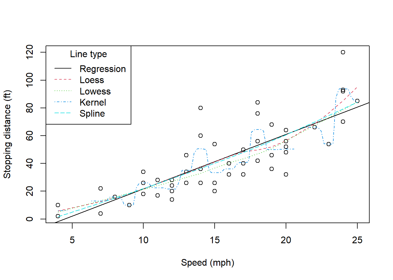
Figure 8.1: to fix
For no other reason than that it is convenient, knots will be placed at days 50, 100, 150, and 200 in our first example. Figure \[WeightLossCubicSpline\] shows a cubic spline fitted using a linear model framework and the parameterisation described in Equation \[TruncatedPowerFunction\].
    WeightLoss$DaysPast50=ifelse(WeightLoss$Days>50,(WeightLoss$Days-50)^3,0)
    WeightLoss$DaysPast100=ifelse(WeightLoss$Days>100,(WeightLoss$Days-100)^3,0)
    WeightLoss$DaysPast150=ifelse(WeightLoss$Days>150,(WeightLoss$Days-150)^3,0)
    WeightLoss$DaysPast200=ifelse(WeightLoss$Days>200,(WeightLoss$Days-200)^3,0)
    WeightLoss.lm = lm(Weight~poly(Days,3)+DaysPast50+DaysPast100+DaysPast150+DaysPast200, data=WeightLoss)
    anova(WeightLoss.lm)
Analysis of Variance Table
Response: Weight
Df Sum Sq Mean Sq F value Pr(>F)
poly(Days, 3) 3 22672 7557 8731.43 <2e-16 ***
DaysPast50 1 0 0 0.26 0.61
DaysPast100 1 1 1 0.82 0.37
DaysPast150 1 0 0 0.21 0.65
DaysPast200 1 0 0 0.03 0.86
Residuals 44 38 1
---
Signif. codes: 0 '***' 0.001 '**' 0.01 '*' 0.05 '.' 0.1 ' ' 1 Days Weight DaysPast50 DaysPast100 DaysPast150 DaysPast200
Days 1.0000 -0.9853 0.8325 0.7447 0.6512 0.5183
Weight -0.9853 1.0000 -0.7338 -0.6356 -0.5395 -0.4190
DaysPast50 0.8325 -0.7338 1.0000 0.9857 0.9385 0.7991
DaysPast100 0.7447 -0.6356 0.9857 1.0000 0.9803 0.8601
DaysPast150 0.6512 -0.5395 0.9385 0.9803 1.0000 0.9314
DaysPast200 0.5183 -0.4190 0.7991 0.8601 0.9314 1.0000As seen, the cubic spline terms add little value to the polynomial
regression model. Also note the use of the cor() command to obtain the
correlation matrix for the variables used in this model. Clearly they
are not orthogonal (independent).
A more robust method for determining the location and number of knots is desirable. R does have some useful commands for creating splines. In Figure \[WeightLossCubicBSpline\] we see how the cubic spline is created using the B-spline parameterisation.
Loading required package: splines attach(WeightLoss)
plot(Days, Weight)
lines(Days, fitted(lm(Weight~poly(Days,3))), lty=2)
lines(Days, fitted(lm(Weight~bs(Days, df=10))), col=2)
legend("topright", c("polynomial fit", "B-spline fit"), lty=c(2,1), col=c(1,2))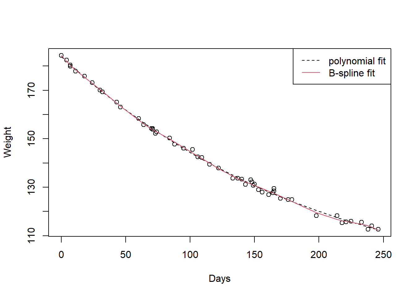
Figure 8.2: to fix
The suitability of the B-spline fit for this data is somewhat arguable. There is a definite risk of overfitting the data by adding too many parameters to our model. The fit of the B-spline is given in Figure \[WeightLossBSpline\] for completeness,
Call:
lm(formula = Weight ~ bs(Days, df = 10), data = WeightLoss)

Residuals:
   Min     1Q Median     3Q    Max
-1.554 -0.440  0.057  0.456  1.991

Coefficients:
                    Estimate Std. Error t value Pr(>|t|)
(Intercept)          184.460      0.800   230.6  < 2e-16 ***
bs(Days, df = 10)1    -5.765      1.560    -3.7  0.00064 ***
bs(Days, df = 10)2   -14.019      1.229   -11.4  2.7e-14 ***
bs(Days, df = 10)3   -28.460      1.230   -23.1  < 2e-16 ***
bs(Days, df = 10)4   -37.379      1.197   -31.2  < 2e-16 ***
bs(Days, df = 10)5   -47.453      1.352   -35.1  < 2e-16 ***
bs(Days, df = 10)6   -53.219      0.973   -54.7  < 2e-16 ***
bs(Days, df = 10)7   -59.186      1.209   -48.9  < 2e-16 ***
bs(Days, df = 10)8   -69.159      1.726   -40.1  < 2e-16 ***
bs(Days, df = 10)9   -69.303      1.375   -50.4  < 2e-16 ***
bs(Days, df = 10)10  -72.073      1.144   -63.0  < 2e-16 ***
---
Signif. codes:  0 '***' 0.001 '**' 0.01 '*' 0.05 '.' 0.1 ' ' 1

Residual standard error: 0.901 on 41 degrees of freedom
Multiple R-squared:  0.999, Adjusted R-squared:  0.998
F-statistic: 2.79e+03 on 10 and 41 DF,  p-value: <2e-16
but note that this does not show us the location of the knots chosen.
8.3 Other smoothers
There are a number of ways of creating a smooth curve to represent a
series of points. We have for example already used the lowess()
function to generate curves in
Example \[ExampleBeetles\] without necessarily understanding its
behaviour. In fact, this function has been superceded by the loess()
function — the differences being in the default arguments. These
functions create curves using locally weighted polynomial regression.
A locally weighted polynomial regression algorithm assigns weights to
each observation for each regression model fitted. A series of these
models is required to find the overall set of smoothed values for the
relationship being examined. Points are weighted by their proximity to
the x value being modelled, with those observations that are not
considered ‘local’ being ignored. This is often known as using points
within a ‘window’. Altering the size of this window is a key element
when choosing the particular smoothed curve that is generated by this
algorithm. Some experimentation of the arguments used for either the
lowess() or loess() commands is warranted.
The ksmooth() function uses a kernel smoother to find particular
values of the response variable using: \[\label{MASS9.2}
\hat{y_i} = \frac{
\sum_{j=1}^n {
y_j K(\frac{x_i-x_j}{b}) }}{
\sum_{j=1}^n {
K(\frac{x_i-x_j}{b}) }}\] where b is the band width parameter and K
is a kernel function, based in this case on the standard normal
distribution. Consideration of b and K are beyond the scope of this
discussion. See (Venables and Ripley 2002) and references therein for more detail, but note
that the help page for this function points towards “better smoothers"
without actually specifying them.
A scatter plot smoother available using the command finds a smooth curve for n observations based on minimising:\[\sum_i {w_i \left[y_i - f(x_i)\right]^2 } +\lambda \int {\left(f^{\prime\prime}(x) \right)^2.dx}\] Users can specify the value of \(\lambda\) or the equivalent degrees of freedom. The smoother will optimise the value of \(\lambda\) if it is not specified.
8.3.1 Example: Stopping distances of cars
The example commands given for the cars dataset in the datasets
package, and the loess() function inspired this example. The data are
for 50 cars and we have just the speed and the distance taken to stop.
Figure \[CarsPlot\] shows the raw data and the smoothed series using
the default settings for the loess() function. In particular, the
window used by the span argument of span=0.75 which is not given
here is necessary. Failure to smooth the series this much does lead to a
model that is illogical. Investigating this is left as an exercise.
The default smoothed functions for the loess(), lowess(),
ksmooth(), and functions are compared with the simple linear
regression model line in this exhibit. Judgement is needed to informally
choose among the various options for representing this relationship. We
could think of looking at residual plots etc. but more importantly we
need to consider the relationship being modelled and whether we have
over-fitted the data. This should be fairly obvious for the kernel
smoother in this example.
\[CarsPlot\]
    data(cars)
    plot(cars, xlab = "Speed (mph)", ylab = "Stopping distance (ft)")
    abline(lm(dist~speed, data=cars))
    lines(cars$speed, predict(loess(dist~speed, data=cars)), col = 2, lty=2)
    lines(lowess(cars$dist~cars$speed), col = 3, lty=3)
    lines(ksmooth(cars$speed, cars$dist, kernel="normal"), col = 4, lty=4)
    lines(smooth.spline(cars$dist~cars$speed), col = 5, lty=5)
    legend("topleft", c("Regression", "Loess", "Lowess", "Kernel", "Spline"), col=1:5, lty=1:5, title="Line type")
Figure 8.3: to fix
Loading required package: gamLoading required package: foreach
Attaching package: 'foreach'The following objects are masked from 'package:purrr':
accumulate, whenLoaded gam 1.22-78.4 The generalised additive model (GAM)
A generalised additive model takes the additive model given above and allows for the response variable to come from a distribution other than normal. For example, a cubic spline (Equation \[TruncatedPowerFunction\] with degree 3) assuming normal response data would be: \[y_i \sim Normal\left[ \beta_0 + \beta_1 x_i +\beta_2 x_i^2 +\beta_3 x_i^3 + \sum_{k=1}^K {b_{3k} (x_i- \kappa_k)_+^3 } , \quad \sigma_\varepsilon ^2\right]\]
The general linear model for Poisson data is \[y_i \sim Poisson\left[ \exp\left( \boldsymbol{X}\boldsymbol{\beta} \right)_i \right]\] To convert this to a generalised additive model (GAM) for Poisson data we need to replace the design matrix \(\boldsymbol{X}\) by the matrix representation of the additive model chosen from among those given earlier (or others).
For a binomially distributed response we might use the GLM \[{\rm logit}(p) = \alpha + \sum_{j=1}^J {\beta_j x_j}\] or the GAM \[{\rm logit}(p) = \alpha + \sum_{j=1}^J {f_j (x_j)}\]
The upshot is that all we need to do to fit a GAM in a practical sense is to replace the standard right hand side of any GLM, by that appropriate for smoothing under an additive model framework. Let’s now look at some examples.
8.4.1 Example: Weight loss of an obese male (Example 1.2.1 revisited)
The generalised additive model framework allows the response variable to follow a normal distribution. We therefore use the Weight Loss data again for illustrative purposes. The polynomial model and a generalised additive model are shown in Figure \[WeightLossGAM\].
Call:
lm(formula = Weight ~ poly(Days, 3), data = WeightLoss)

Residuals:
    Min      1Q  Median      3Q     Max
-2.1822 -0.6031  0.0015  0.4909  2.3369

Coefficients:
               Estimate Std. Error t value Pr(>|t|)
(Intercept)     142.248      0.125 1134.58   <2e-16 ***
poly(Days, 3)1 -148.490      0.904 -164.24   <2e-16 ***
poly(Days, 3)2   24.879      0.904   27.52   <2e-16 ***
poly(Days, 3)3   -1.983      0.904   -2.19    0.033 *
---
Signif. codes:  0 '***' 0.001 '**' 0.01 '*' 0.05 '.' 0.1 ' ' 1

Residual standard error: 0.904 on 48 degrees of freedom
Multiple R-squared:  0.998, Adjusted R-squared:  0.998
F-statistic: 9.25e+03 on 3 and 48 DF, p-value: <2e-16Loading required package: mgcvThis is mgcv 1.9-4. For overview type '?mgcv'.
Family: gaussian
Link function: identity

Formula:
Weight ~ s(Days)

Parametric coefficients:
            Estimate Std. Error t value Pr(>|t|)
(Intercept)  142.248      0.125    1138   <2e-16 ***
---
Signif. codes:  0 '***' 0.001 '**' 0.01 '*' 0.05 '.' 0.1 ' ' 1

Approximate significance of smooth terms:
         edf Ref.df    F p-value
s(Days) 5.32   6.44 4331  <2e-16 ***
---
Signif. codes:  0 '***' 0.001 '**' 0.01 '*' 0.05 '.' 0.1 ' ' 1

R-sq.(adj) =  0.998   Deviance explained = 99.8%
GCV = 0.92482 Scale est. = 0.81235 n = 52[1] 142.9[1] 144.7Either model is useful, but the comparison of AIC values would suggest that neither model has a real advantage. Computationally speaking, the simpler model would be a better option.
8.5 A special note on add-on package options
Please take special note here. The gam and mgcv packages both fit
generalised additive models. Their fitting routines are different; their
functions are different, but many have similar names. Any functions with
the same name will give the same results if the arguments are functional
in both packages. Care is therefore required to ensure the correct
package is active when the model is fitted. Note that the mgcv package
does not use the lo() smoother for example. It does offer some more
advanced functionality that is not present in the gam package so it is
used more commonly from this point onwards.
The detach() command is used prior to the require() command in order
to ensure that both packages are not active at the same time.
8.5.1 Example: AIDS deaths in Australia (Example \[ExampleAids\] revisited)
A generalised linear model for Poisson data was used in
Example \[ExampleAids\]. We can compare this model with the generalised
additive model. Note that use of the gam() function has a family
argument in similar fashion to that used in the glm() function.
Figure \[AidsGLM1\] shows the fit of the GLM and
Figure \[AidsGAM\]
shows that of the GAM.
    data(Aids, package="ELMER")
    Aids.glm<-glm(Deaths~-1+Period,family=poisson,data=Aids)
    summary(Aids.glm)
Call:
glm(formula = Deaths ~ -1 + Period, family = poisson, data = Aids)

Coefficients:
       Estimate Std. Error z value Pr(>|z|)
Period  0.28504    0.00589    48.4   <2e-16 ***
---
Signif. codes:  0 '***' 0.001 '**' 0.01 '*' 0.05 '.' 0.1 ' ' 1

(Dispersion parameter for poisson family taken to be 1)

    Null deviance: 1001.779  on 14  degrees of freedom
Residual deviance:   31.385  on 13  degrees of freedom
AIC: 86.31

Number of Fisher Scoring iterations: 4
Family: poisson
Link function: log

Formula:
Deaths ~ -1 + s(Period)

Approximate significance of smooth terms:
           edf Ref.df Chi.sq p-value
s(Period) 8.83   8.98   2328  <2e-16 ***
---
Signif. codes:  0 '***' 0.001 '**' 0.01 '*' 0.05 '.' 0.1 ' ' 1

R-sq.(adj) =  0.982   Deviance explained = 94.1%
UBRE = 1.1299  Scale est. = 1         n = 14
Note that the y intercept has been explicitly removed from both models
. The marginal improvement of the GAM over the GLM obtained earlier is
shown in
Figure \[AidsCompareGAM\]. This is tested using the anova()
function, but note that we use a likelihood ratio test.
Analysis of Deviance Table

Model 1: Deaths ~ -1 + Period
Model 2: Deaths ~ -1 + s(Period)
  Resid. Df Resid. Dev   Df Deviance Pr(>Chi)
1     13.00       31.4
2      5.17       12.2 7.83     19.2    0.012 *
---
Signif. codes:  0 '***' 0.001 '**' 0.01 '*' 0.05 '.' 0.1 ' ' 1
We can see this improvement in the fit in Figure \[AidsFittedGAM\].
    plot(Deaths~Period, cex.lab=1.5, data=Aids)
    lines(exp(Aids.glm$coef[1]*Aids$Period), lty=2)
    lines(fitted(Aids.gam), col=2)
    legend("bottomright", c("GLM","GAM"),lty=c(2,1), col=c(1,2))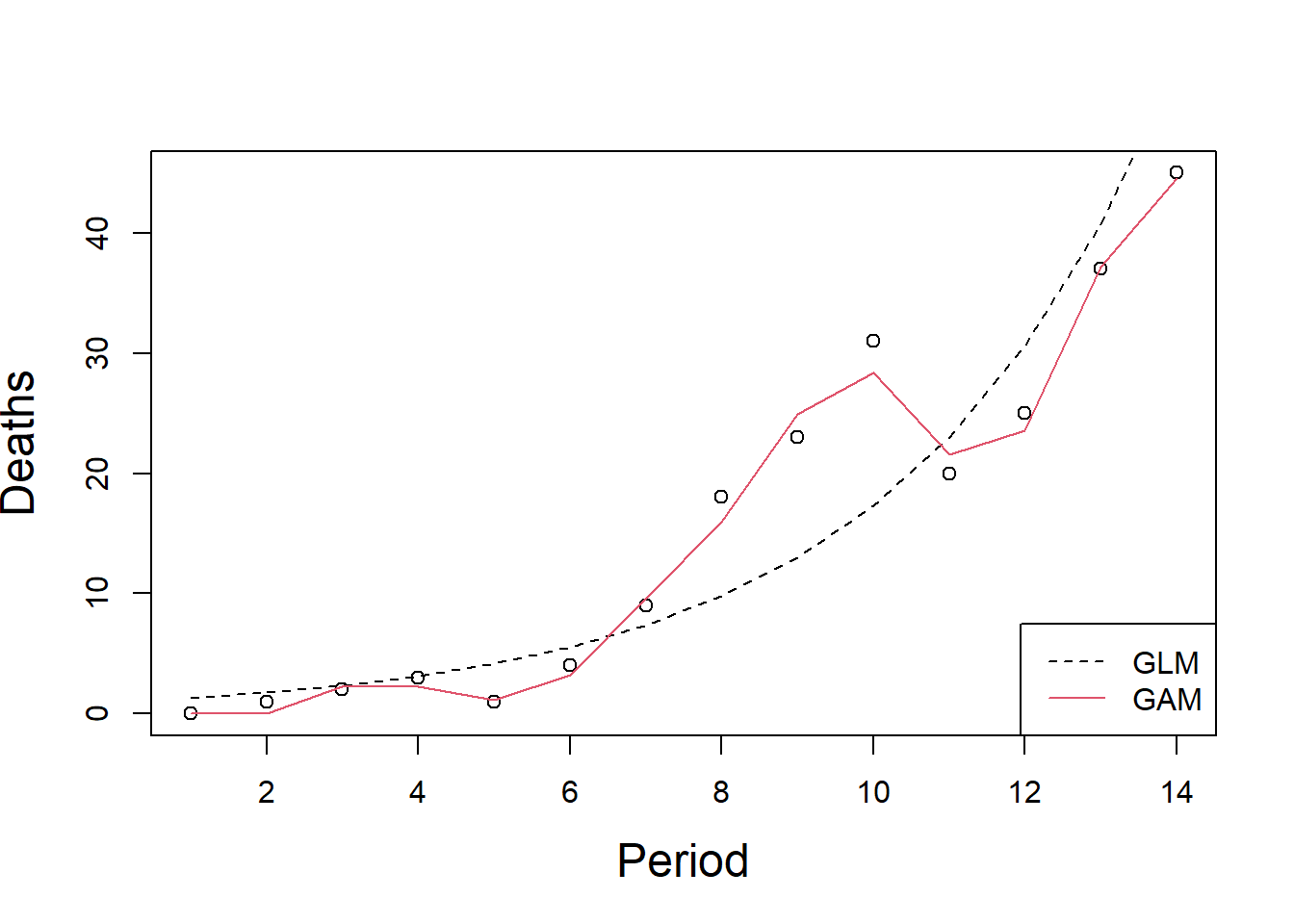
Figure 8.4: to fix
8.5.2 Example: Detection of blood proteins
(Collett and Jemain 1985) used data from an investigation of the relationship between the levels of certain blood proteins and the rate at which red blood cells settle out of the blood (called erythrocyte sedimentation rate or ESR). ESR is easy to measure, so if it is associated with blood protein levels it might provide a useful screening test for diseases which cause a rise in these levels. On the basis that normal individuals would be expected to have an ESR of less than 20mm/hr, we want to know if people with high blood protein levels are more likely to have ESR > 20. Two blood proteins have been recorded in this data set.
In (Godfrey 2012), a logistic regression model was fitted to this data. It is re-presented in Figure \[PlasmaGLM\].
    data(Plasma, package="ELMER")
    Plasma.glm<-glm(ESR~Fibrinogen+Globulin, family=binomial(), data=Plasma)
    summary(Plasma.glm)
Call:
glm(formula = ESR ~ Fibrinogen + Globulin, family = binomial(),
    data = Plasma)

Coefficients:
            Estimate Std. Error z value Pr(>|z|)
(Intercept)  -12.792      5.796   -2.21    0.027 *
Fibrinogen     1.910      0.971    1.97    0.049 *
Globulin       0.156      0.120    1.30    0.193
---
Signif. codes:  0 '***' 0.001 '**' 0.01 '*' 0.05 '.' 0.1 ' ' 1

(Dispersion parameter for binomial family taken to be 1)

    Null deviance: 30.885  on 31  degrees of freedom
Residual deviance: 22.971  on 29  degrees of freedom
AIC: 28.97

Number of Fisher Scoring iterations: 5
We now see (Figure \[PlasmaGAM\]) that a generalised additive model can be fitted to this data, using a smoothed function of each of the two predictor variables.
    #detach("package:gam")
    require(mgcv)
    Plasma.gam1 <-gam(ESR~s(Fibrinogen)+s(Globulin), family=binomial(), data=Plasma)
    summary(Plasma.gam1)
Family: binomial
Link function: logit

Formula:
ESR ~ s(Fibrinogen) + s(Globulin)

Parametric coefficients:
            Estimate Std. Error z value Pr(>|z|)
(Intercept)   -1.684      0.831   -2.03    0.043 *
---
Signif. codes:  0 '***' 0.001 '**' 0.01 '*' 0.05 '.' 0.1 ' ' 1

Approximate significance of smooth terms:
               edf Ref.df Chi.sq p-value
s(Fibrinogen) 2.28   2.85   3.69    0.22
s(Globulin)   1.00   1.00   1.83    0.18

R-sq.(adj) =  0.503   Deviance explained = 48.9%
UBRE = -0.23969  Scale est. = 1         n = 32
Family: binomial
Link function: logit

Formula:
ESR ~ s(Globulin) + s(Fibrinogen)

Parametric coefficients:
            Estimate Std. Error z value Pr(>|z|)
(Intercept)   -1.684      0.831   -2.03    0.043 *
---
Signif. codes:  0 '***' 0.001 '**' 0.01 '*' 0.05 '.' 0.1 ' ' 1

Approximate significance of smooth terms:
               edf Ref.df Chi.sq p-value
s(Globulin)   1.00   1.00   1.83    0.18
s(Fibrinogen) 2.28   2.85   3.69    0.22

R-sq.(adj) =  0.503   Deviance explained = 48.9%
UBRE = -0.23969  Scale est. = 1         n = 32
Note that a second GAM is fitted here using the same two predictors in the alternate order, so that we can confirm that the models are in fact the same.
In Figure \[PlasmaCompare\] we see a likelihood ratio test procedure to evaluate the value of the added complexity introduced by the smoothed functions of our predictors.
Analysis of Deviance Table

Model 1: ESR ~ Fibrinogen + Globulin
Model 2: ESR ~ s(Fibrinogen) + s(Globulin)
  Resid. Df Resid. Dev   Df Deviance Pr(>Chi)
1      29.0       23.0
2      27.7       15.8 1.28     7.19    0.011 *
---
Signif. codes:  0 '***' 0.001 '**' 0.01 '*' 0.05 '.' 0.1 ' ' 1
We can investigate the nature of the smoothed functions of the two predictors in our model, shown in Figure \[PlasmaSmoothers\]

Figure 8.5: to fix
We see that the smoothed functions of the predictors is not dependent on
the ordering of the predictors in the two models. We also see that the
functions are smooth, but that the function for Fibrinogen is not
monotonic. This lack of monotonicity is not a problem in a mathematical
sense, but is problematic in a practical sense. We need to determine if
this relationship makes sense medically speaking before determining this
model’s value. If the model does not make medical sense then we need to
force the model to exclude the possibility of a decrease in the smoothed
function. Such manipulation may require manual creation of the smoothed
function rather than reliance on the s() function used here, but we
also have a risk of over-fitting to watch out for when we fit any GAM.
The mgcv package has a convenience function for checking the validity
of the fitted model. See its use in
Figure \[PlasmaGAMCheck\].
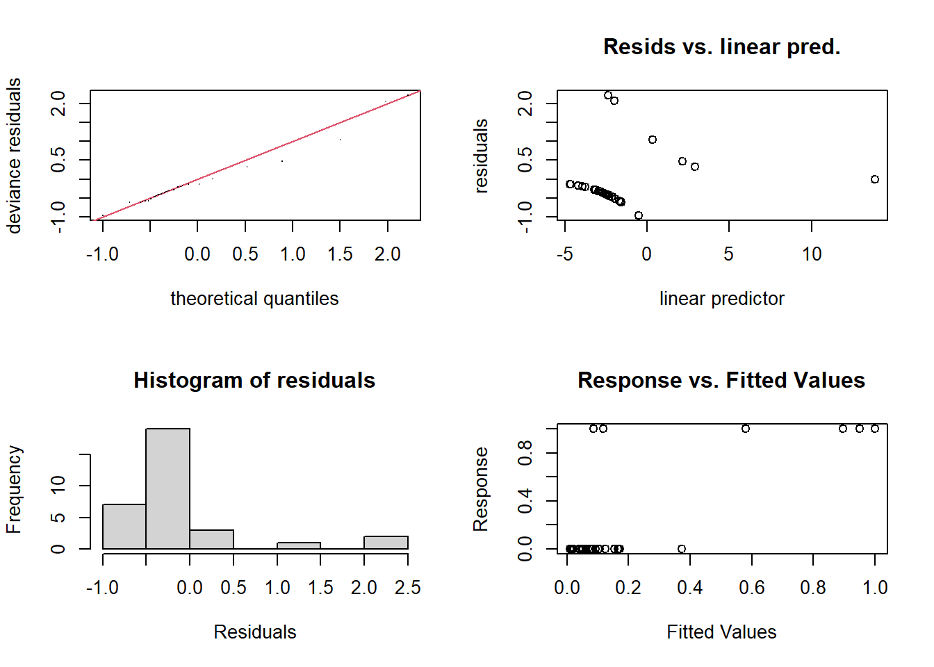
Figure 8.6: to fix
Method: UBRE   Optimizer: outer newton
full convergence after 9 iterations.
Gradient range [-6.312e-07,5.544e-08]
(score -0.2397 & scale 1).
Hessian positive definite, eigenvalue range [6.312e-07,0.01464].
Model rank =  19 / 19

Basis dimension (k) checking results. Low p-value (k-index<1) may
indicate that k is too low, especially if edf is close to k'.

                k'  edf k-index p-value
s(Fibrinogen) 9.00 2.28    1.07    0.56
s(Globulin)   9.00 1.00    0.95    0.30
Given we have a small number of data points and the response is binary, it is no surprise at all that the residual analysis plots are highlighting some strange behaviour.
Finally, we see the fitted values from both the GLM and GAM plotted against the two predictors in Figure \[PlasmaFitted\]. The lack of monotonicity of the smoothed function of Fibrinogen does not negatively impact on the nature of the relationship fitted by the GAM.
    par(mfrow=c(2,2))
    plot(fitted(Plasma.glm)~Fibrinogen, data=Plasma)
    plot(fitted(Plasma.glm)~Globulin, data=Plasma)
    plot(fitted(Plasma.gam1)~Fibrinogen, data=Plasma)
    plot(fitted(Plasma.gam1)~Globulin, data=Plasma)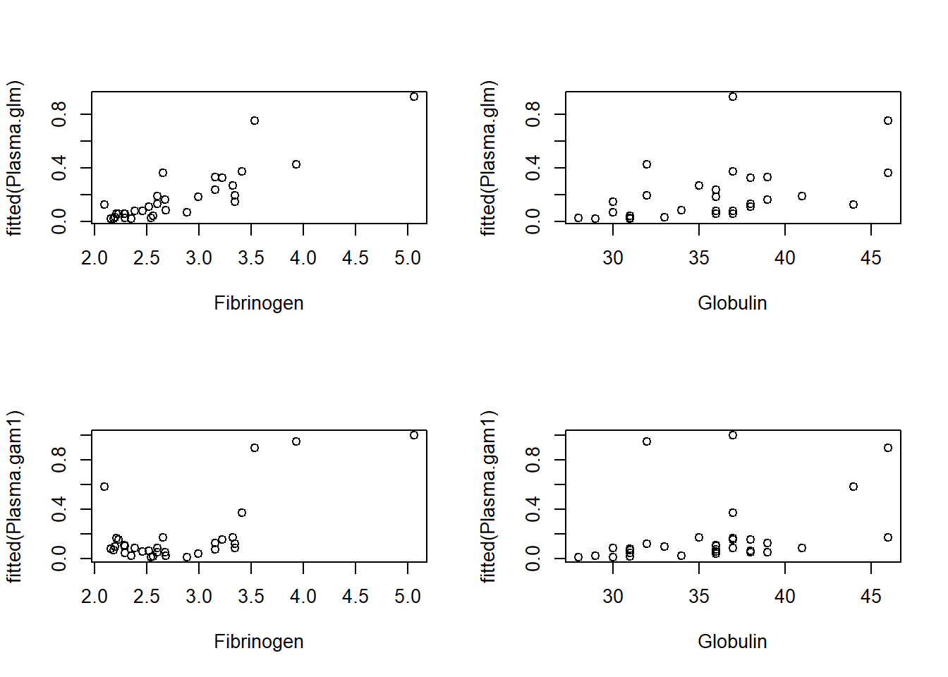
Figure 8.7: to fix
Finding a more suitable plot to elucidate the relationship among these variables is left as an exercise.
8.6 Exercises
8.6.1
Sometimes a smoother can give misleading results, especially when the
number of points is small. Investigate the fitted values from the model
for Beetle mortality
(Figure \[BeetlesIntervals\]), apply a smoother (lowess() for
example), and see what occurs.
8.6.2
Re-consider the data used for Example 1.3.1 and the default settings for each of the smoothers. Alter the settings in order to monitor the sensitivity of each smoother.
8.6.3
The plots in Figure \[PlasmaFitted\] are not especially useful for showing the overall relationship among these three variables. Find a more suitable plot that could be used in a presentation.
8.6.4
Example 1.2.1 used an arbitrary set of knot points. Repeat this analysis using knots at 75, 125, and 175. How much impact does the choice of knot points matter in this context?