Lecture 19 Analysis of Covariance
19.1 Analysis of Covariance - ANCOVA
We consider the situation where we want to quantify the effect of a categorical variable after first adjusting for the effect of a covariate. This is called ANCOVA - analysis of covariance.
In the following example, we want to know whether the layout of shops (called ‘Arrngmt’ : shop arrangement) makes a difference to the profitability of those shops. Three different arrangements were tried, in different branches of a chain store. In order to answer the question we need to first adjust for the covariate effect ‘RtailSpc’ (retail space – the floor area of the shop).
  Arrngmt Shop RtailSpc Profit Arr1 Arr2
1       1    1     26.8   22.2    1    0
2       1    2     38.1   25.2    1    0
3       1    3     44.5   26.8    1    0
4       1    4     25.6   33.3    1    0
5       1    5     12.0   15.7    1    0
6       2    6     40.7   22.5    0    1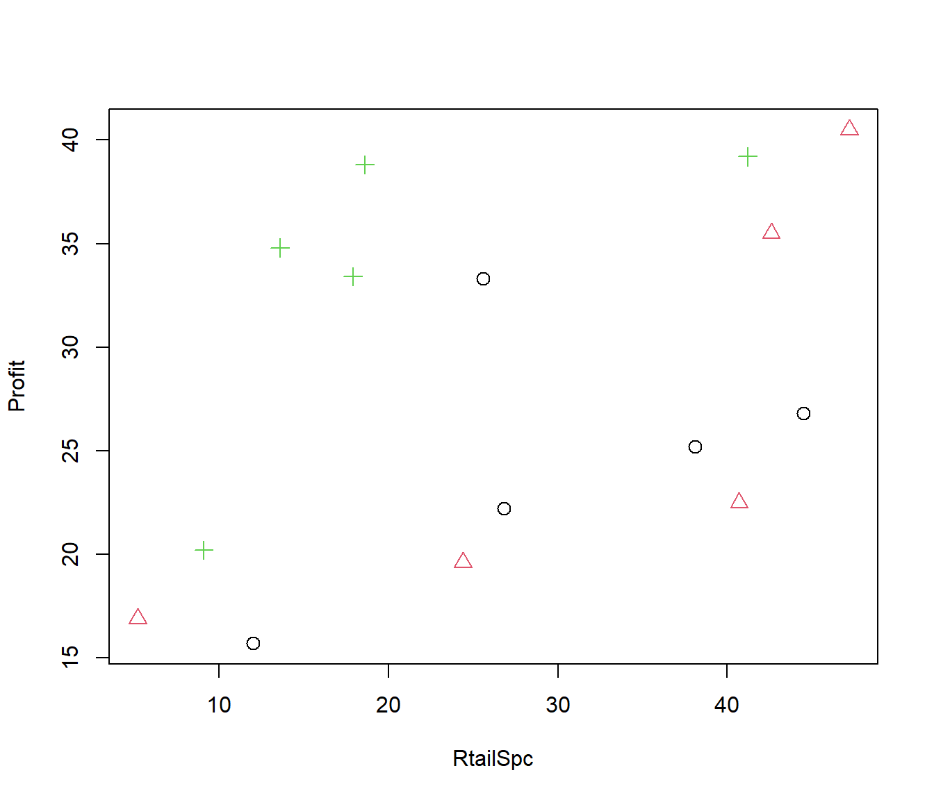
We fit a linear model to first adjust for the covariate, then include the factor.
Retail.lm1 = lm(Profit ~ RtailSpc, data = Retail)
Retail.lm2 = lm(Profit ~ RtailSpc + as.factor(Arrngmt), data = Retail)
summary(Retail.lm2)
Call:
lm(formula = Profit ~ RtailSpc + as.factor(Arrngmt), data = Retail)

Residuals:
   Min     1Q Median     3Q    Max
-8.577 -3.520 -1.374  4.169 10.218

Coefficients:
                    Estimate Std. Error t value Pr(>|t|)
(Intercept)          12.5834     4.6353   2.715  0.02012 *
RtailSpc              0.4101     0.1261   3.253  0.00769 **
as.factor(Arrngmt)2   1.2856     3.9508   0.325  0.75099
as.factor(Arrngmt)3  12.4620     4.1086   3.033  0.01138 *
---
Signif. codes:  0 '***' 0.001 '**' 0.01 '*' 0.05 '.' 0.1 ' ' 1

Residual standard error: 6.225 on 11 degrees of freedom
Multiple R-squared:  0.5885,    Adjusted R-squared:  0.4762
F-statistic: 5.243 on 3 and 11 DF, p-value: 0.01724Analysis of Variance Table
Model 1: Profit ~ RtailSpc
Model 2: Profit ~ RtailSpc + as.factor(Arrngmt)
Res.Df RSS Df Sum of Sq F Pr(>F)
1 13 836.56
2 11 426.24 2 410.32 5.2945 0.02451 *
---
Signif. codes: 0 '***' 0.001 '**' 0.01 '*' 0.05 '.' 0.1 ' ' 1We see that the Profit is definitely related to RtailSpc, and there seems to be a significant difference between arrangements 1 and 3, but not between arrangements 1 and 2.
The anova test enables us to average the effect of the different levels of Arrngmt and conclude that, overall, Arrngment is significantly related to Profit.
19.1.1 Is there an interaction ?
We may wonder if some store arrangements make better use of space than others. That is, if the relationship between Profit and RtailSpc is altered, depending on what arrangement is being used. This means fitting an interaction model.
Call:
lm(formula = Profit ~ RtailSpc * as.factor(Arrngmt), data = Retail)

Residuals:
   Min     1Q Median     3Q    Max
-8.735 -3.176 -1.748  3.747  9.668

Coefficients:
                             Estimate Std. Error t value Pr(>|t|)
(Intercept)                   16.8420     8.4331   1.997   0.0769 .
RtailSpc                       0.2652     0.2680   0.990   0.3482
as.factor(Arrngmt)2           -5.4642    10.9005  -0.501   0.6282
as.factor(Arrngmt)3            8.2707    10.4725   0.790   0.4500
RtailSpc:as.factor(Arrngmt)2   0.2226     0.3310   0.673   0.5181
RtailSpc:as.factor(Arrngmt)3   0.1415     0.3809   0.371   0.7189
---
Signif. codes:  0 '***' 0.001 '**' 0.01 '*' 0.05 '.' 0.1 ' ' 1

Residual standard error: 6.715 on 9 degrees of freedom
Multiple R-squared:  0.6082,    Adjusted R-squared:  0.3905
F-statistic: 2.794 on 5 and 9 DF, p-value: 0.08575Analysis of Variance Table
Model 1: Profit ~ RtailSpc + as.factor(Arrngmt)
Model 2: Profit ~ RtailSpc * as.factor(Arrngmt)
Res.Df RSS Df Sum of Sq F Pr(>F)
1 11 426.24
2 9 405.84 2 20.41 0.2263 0.8019We see that the interaction terms are not significant, whether individually (in terms of slopes) or together (in terms of the ANOVA).
19.1.2 A Plot with Separate Lines and Symbols
You can use the following code to plot a response variable Y versus a covariate X with a group variable (factor) G
library(ggplot2)
Retail |>
    ggplot(aes(x = RtailSpc, y = Profit, group = Arrngmt)) + geom_point() + geom_smooth(method = "lm",
    se = FALSE)
`geom_smooth()` using formula = 'y ~ x'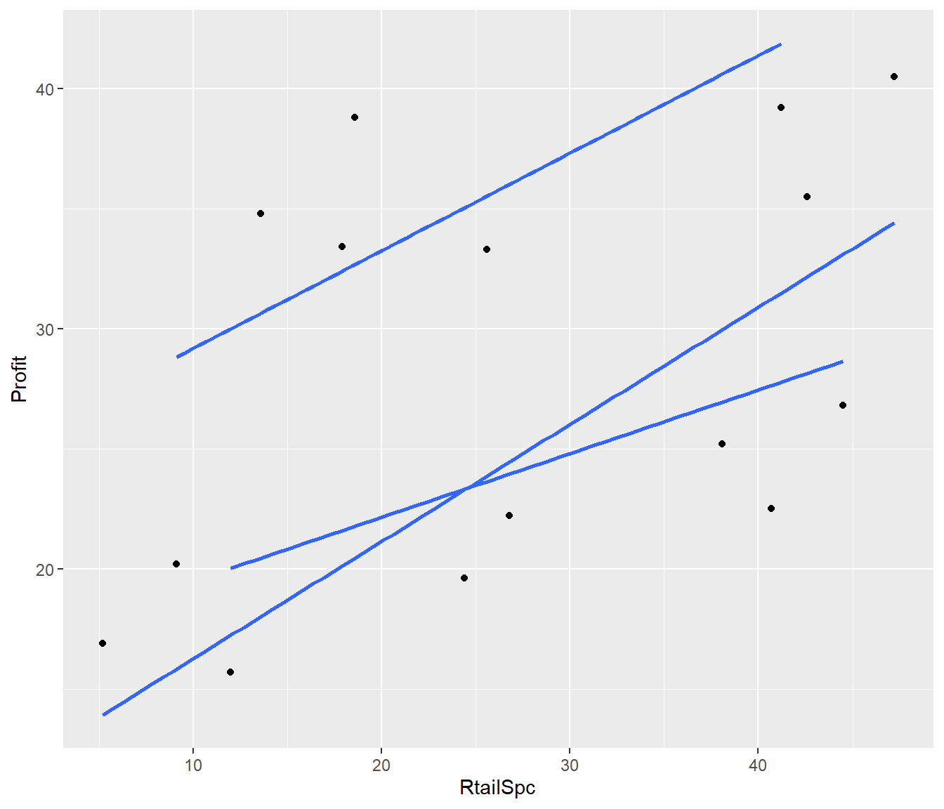
We see from the plot that allows for interaction, that there is little difference in slope between the three groups. If we assume parallel lines then the lines for Arrngmt 1 and 2 are very close together.
19.1.3 Writing down equations from the coefficients
Using the Summary(Retail.lm2) or the following coef(Retail.lm2) we can write down the equations for the regression lines for each group in the case of parallel lines.
For Parallel Lines
        (Intercept)            RtailSpc as.factor(Arrngmt)2 as.factor(Arrngmt)3
         12.5833878           0.4100888           1.2855672          12.4620281
For Arrangement 1, the baseline group, the equation is \[(1) ~~~~~~~ Profit = 12.583 + 0.410 \times RtailSpc \] For Arrangement 2 and 3
\[(2) ~~~~~~~ Profit = (12.583 + 1.286) + 0.410\times RtailSpc \] \[ ~~~~~~~~~~~~~~ = 13.869 + 0.410\times RtailSpc \]
\[(3) ~~~~~~~ Profit =(12.583 + 12.462) + 0.410\times RtailSpc \] \[~~~~~~~~~~~~ = 25.045 + 0.410\times RtailSpc \] For Non-Parallel Lines
                 (Intercept)                     RtailSpc
                  16.8419692                    0.2652391
         as.factor(Arrngmt)2          as.factor(Arrngmt)3
                  -5.4641672                    8.2706914
RtailSpc:as.factor(Arrngmt)2 RtailSpc:as.factor(Arrngmt)3
                   0.2226496                    0.1415009
For the model with an interaction the equations are
\[(Int1) ~~~~~~~ Profit = 16.842 + 0.265 \times RtailSpc \]
\[(Int2) ~~~~~~~ Profit = (16.842 -5.464) + (0.265+ 0.223)\times RtailSpc \] \[ ~~~~~~~~~~~~~~~~ = 11.378 + 0.488\times RtailSpc \] \[(Int3) ~~~~~~~~ Profit = (16.842+ 8.271) + (0.265+ 0.142) \times RtailSpc \] \[ ~~~~~~~~~~~~~~~~ = 25.113 + 0.407\times RtailSpc \]
In the case of non-parallel lines we can check the equations by subsetting the variables. But we cannot do this for the parallel-line model.
Call:
lm(formula = Profit[Arrngmt == 2] ~ RtailSpc[Arrngmt == 2], data = Retail)

Coefficients:
           (Intercept)  RtailSpc[Arrngmt == 2]
               11.3778                  0.4879
19.2 Exercise
Read in the NSRent2021.csv data. The response variable is rent, and predictor variables are bedrooms and bathrooms.
- Plot to see whether the relationship between rent and bedrooms is parallel if the number of bathrooms is treated as a factor. (Note more recent houses tend to have more bathrooms)
NSrent21 |>
    ggplot(aes(x = bedrooms, y = rent, group = bathrooms)) + geom_point() + geom_smooth(method = "lm",
    se = FALSE)
`geom_smooth()` using formula = 'y ~ x'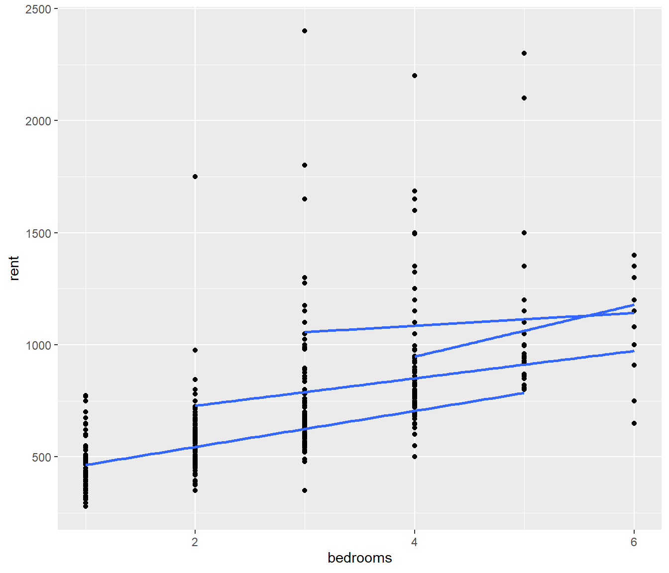
- Fit a parallel-lines model
lm1 = lm(rent~ bedrooms + as.factor(bathrooms))
Assuming a two-bathroom house, write down the equation relating the expected rent to the number of bedrooms.
- Fit an interaction model
lm2 = lm(rent~ bedrooms * as.factor(bathrooms))
Is the interaction model significantly better than a parallel-lines model?
Calculate the formula for the lines relating expected rent to number of bedrooms for one- and two- bathroom houses. Check your calculation by subseting the data (e.g. [bathrooms==2]) .
What is the expected rent for a house with 3 bedrooms and 2 bathrooms?
Solution
  bedrooms bathrooms rent
1        1         1  280
2        1         1  280
3        1         1  295
4        1         1  295
5        1         1  310
6        1         1  320
Call:
lm(formula = rent ~ bedrooms + as.factor(bathrooms), data = NSrent)

Residuals:
    Min      1Q  Median      3Q     Max
-462.28  -75.85  -19.69   33.51 1617.35

Coefficients:
                      Estimate Std. Error t value Pr(>|t|)
(Intercept)            400.103     19.318  20.711  < 2e-16 ***
bedrooms                73.195      7.866   9.306  < 2e-16 ***
as.factor(bathrooms)2  162.966     18.115   8.996  < 2e-16 ***
as.factor(bathrooms)3  373.011     30.733  12.137  < 2e-16 ***
as.factor(bathrooms)4  309.962     60.276   5.142 3.52e-07 ***
---
Signif. codes:  0 '***' 0.001 '**' 0.01 '*' 0.05 '.' 0.1 ' ' 1

Residual standard error: 172.7 on 706 degrees of freedom
Multiple R-squared:  0.5311,    Adjusted R-squared:  0.5284
F-statistic: 199.9 on 4 and 706 DF,  p-value: < 2.2e-16
Call:
lm(formula = rent ~ bedrooms * as.factor(bathrooms), data = NSrent)

Residuals:
    Min      1Q  Median      3Q     Max
-392.95  -70.89  -19.89   34.77 1610.27

Coefficients:
                               Estimate Std. Error t value Pr(>|t|)
(Intercept)                     384.190     22.869  16.799  < 2e-16 ***
bedrooms                         80.348      9.599   8.371 3.09e-16 ***
as.factor(bathrooms)2           222.068     60.290   3.683 0.000248 ***
as.factor(bathrooms)3           586.648    163.909   3.579 0.000368 ***
as.factor(bathrooms)4           100.400    375.193   0.268 0.789088
bedrooms:as.factor(bathrooms)2  -19.189     17.958  -1.069 0.285630
bedrooms:as.factor(bathrooms)3  -51.662     37.390  -1.382 0.167495
bedrooms:as.factor(bathrooms)4   35.390     70.561   0.502 0.616141
---
Signif. codes:  0 '***' 0.001 '**' 0.01 '*' 0.05 '.' 0.1 ' ' 1

Residual standard error: 172.7 on 703 degrees of freedom
Multiple R-squared:  0.5331,    Adjusted R-squared:  0.5285
F-statistic: 114.7 on 7 and 703 DF, p-value: < 2.2e-16Analysis of Variance Table
Model 1: rent ~ bedrooms + as.factor(bathrooms)
Model 2: rent ~ bedrooms * as.factor(bathrooms)
Res.Df RSS Df Sum of Sq F Pr(>F)
1 706 21046994
2 703 20955432 3 91563 1.0239 0.3814
Call:
lm(formula = rent[bathrooms == 1] ~ bedrooms[bathrooms == 1],
    data = NSrent)

Residuals:
    Min      1Q  Median      3Q     Max
-275.23  -45.23   -9.89   34.77 1205.11

Coefficients:
                         Estimate Std. Error t value Pr(>|t|)
(Intercept)                384.19      13.03   29.48   <2e-16 ***
bedrooms[bathrooms == 1]    80.35       5.47   14.69   <2e-16 ***
---
Signif. codes:  0 '***' 0.001 '**' 0.01 '*' 0.05 '.' 0.1 ' ' 1

Residual standard error: 98.39 on 443 degrees of freedom
Multiple R-squared:  0.3275,    Adjusted R-squared:  0.326
F-statistic: 215.7 on 1 and 443 DF,  p-value: < 2.2e-16
Call:
lm(formula = rent[bathrooms == 2] ~ bedrooms[bathrooms == 2],
    data = NSrent)

Residuals:
    Min      1Q  Median      3Q     Max
-323.21 -110.89  -59.73   34.20 1610.27

Coefficients:
                         Estimate Std. Error t value Pr(>|t|)
(Intercept)                606.26      75.06   8.077 5.91e-14 ***
bedrooms[bathrooms == 2]    61.16      20.42   2.995  0.00309 **
---
Signif. codes:  0 '***' 0.001 '**' 0.01 '*' 0.05 '.' 0.1 ' ' 1

Residual standard error: 232.3 on 202 degrees of freedom
Multiple R-squared:  0.04252,   Adjusted R-squared:  0.03778
F-statistic: 8.97 on 1 and 202 DF, p-value: 0.003088(Intercept)
789.7348