Lecture 20 Diagnostics and Multiple Comparisons for Oneway ANOVA
This lecture follows on from last time when we used a factor as a predictor in our model.
20.1 Diagnostics for Caffeine Data
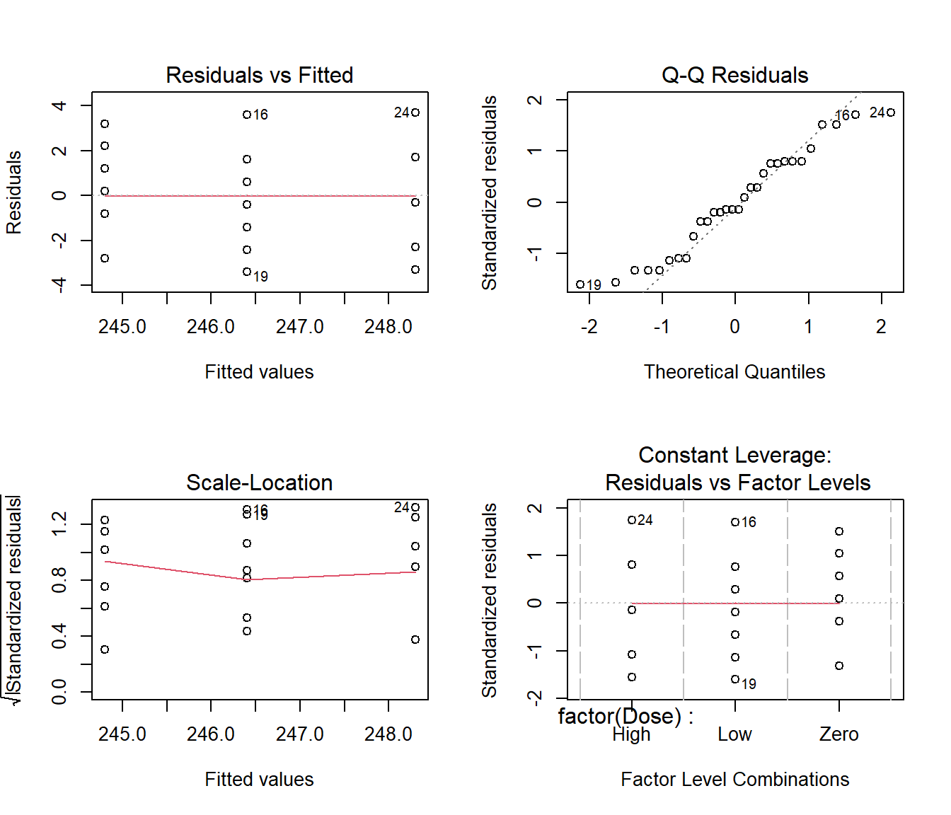
We have tested whether the speed of students’ finger tapping is related to the caffeine dose received. As usual, the validity of our conclusions is contingent on the adequacy of the fitted model. We should therefore inspect standard model diagnostics.
## Caffeine <- read.csv(file = "caffeine.csv", header = T)

Caffeine.lm = lm(Taps ~ factor(Dose), data = Caffeine)

par(mfrow = c(2, 2))
plot(Caffeine.lm)
20.2 Tests for Heteroscedasticity
These are the same as for binary variables. The hypotheses for this test are:
\(H_0\): error variance constant across groups, versus
\(H_1\): error variance not constant across groups
Rejecting the null means that the equal variance assumption is violated.
As before, we can check using Bartlett’s test (if we think the residuals look reasonably normal) or Levene’s test (needs the car package).
    Bartlett test of homogeneity of variances

data:  Taps by Dose
Bartlett's K-squared = 0.18767, df = 2, p-value = 0.9104Levene's Test for Homogeneity of Variance (center = median)
Df F value Pr(>F)
group 2 0.2819 0.7565
27 The P-value for both these tests is large, which confirms that, for the caffeine data, we have no reason to doubt the constant variance assumption.
20.3 Multiple Comparisons
In a factor model, the overall importance of the factor should be assessed by performing an F test.
But sometimes we may have a particular question relating to the relative outcomes at various factor levels that also requires testing. This is OK.
If a factor is found to be significant, some researchers like to compare the relative outcomes between many pairs of factor levels.
This is sometimes referred to as post hoc testing. Post hoc means “after this” in Latin. Thus it is something you do after establishing that the means are not all equal.
This should be done with care…
20.3.1 Caffeine Data Revisited
The parameter estimates for the caffeine data model were as follows:
            Estimate Std. Error    t value     Pr(>|t|)
(Intercept)    248.3  0.7047458 352.325610 5.456621e-51
DoseLow         -1.9  0.9966611  -1.906365 6.729867e-02
DoseZero        -3.5  0.9966611  -3.511725 1.584956e-03
Due to the treatment constraint, the estimates \(\hat \alpha_2 = 1.6\) and \(\hat \alpha_3 = 3.5\) represent respectively the difference in mean response between the low dose and control groups, and between the high dose and control groups.
Having found that Dose is statistically significant, we can investigate where the differences in mean response lie.
We could compare factor level means by formal tests:
Is the mean response at low level different from the control group? A t-test of \(H_0\): \(\alpha_2 = 0\) versus \(H_1\): \(\alpha_2 \ne 0\) retains \(H_0\) (\(P=0.12\)); i.e. no difference between low dose and control groups
Is the mean response at high level different from the control group? A t-test of \(H_0\): \(\alpha_3 = 0\) versus \(H_1\): \(\alpha_3 \ne 0\) rejects \(H~0\) (\(P=0.002\)); ie. there is a difference between high and control groups.
20.3.2 The Multiple Comparisons Problem
In the analysis below, the intercept has been dropped from the model. That means the confidence intervals for the coefficients are in fact confidence intervals for the mean Taps at each dose level. We see that the CIs for \(\mu_1\) and for \(\mu_2\) overlap, but the CIs for \(\mu_1\) and \(\mu_3\) do not overlap. So can we conclude that this is where the significant F-value comes from?
Call:
lm(formula = Taps ~ 0 + Dose, data = Caffeine)

Residuals:
   Min     1Q Median     3Q    Max
-3.400 -2.075 -0.300  1.675  3.700

Coefficients:
         Estimate Std. Error t value Pr(>|t|)
DoseHigh 248.3000     0.7047   352.3   <2e-16 ***
DoseLow  246.4000     0.7047   349.6   <2e-16 ***
DoseZero 244.8000     0.7047   347.4   <2e-16 ***
---
Signif. codes:  0 '***' 0.001 '**' 0.01 '*' 0.05 '.' 0.1 ' ' 1

Residual standard error: 2.229 on 27 degrees of freedom
Multiple R-squared:  0.9999,    Adjusted R-squared:  0.9999
F-statistic: 1.223e+05 on 3 and 27 DF, p-value: < 2.2e-16 2.5 % 97.5 %
DoseHigh 246.854 249.746
DoseLow 244.954 247.846
DoseZero 243.354 246.246The problem is that there is not a precise equivalence between a significant F-test result (judged as at the 5% significance level) and what one might think by looking at the so-called 95% confidence intervals. There is a technical issue called the Multiple Comparisons Problem.
This relates to the fact that if we are comparing three group means, then we are making three different two-group comparisons (Zero-Low, Zero-High, Low-High).
So even if H0 is true (i.e. the only differences that show up between group results are due to luck), then we have three chances of one of those luck results appearing significant at the 5% level.
If those three chances were independent (like tickets in three different raffles) then we would have to say that the probability of getting at least one result “significant” is nearly three times greater (closer to 15%). This is unacceptable.
Our situation is somewhat more complicated as our three comparisons are not independent (and hence neither are our three chances). But nevertheless the fact is that we have close to three times the chance of getting at least one significant two-group comparison just by luck.
So our 5% significance rule for Type I error goes out the window.
If we were comparing four groups we would have six different inter-group comparisons. If we performed two-group comparisons between every pair of factor levels for a factor with 20 levels, then we would perform 190 tests. In that case even if \(H_0\) is true we would expect to get \(0.05\times 190\) =9.5 positive tests.
From all this we see that that the conclusion from CIs for the means may not match up with the conclusion from an F test:
• if we have two non-overlapping confidence intervals then this usually (but not always) indicates that the two group means \(\mu_i\) and \(\mu_j\) (say) are different.
• if we have overlapping confidence intervals then this usually (but not always) indicates that two group means \(\mu_i\) and \(\mu_j\) do not differ.
20.3.3 Solution to the multiple comparisons problem
So how do we fix things so that “chance” means the same thing in the CIs as it does in the overall F test?
The answer is to use one of a collection of methods called Post hoc analyses.
20.3.4 Bonferroni Correction for error inflation
The most common approach is to adjust the significance levels using Bonferroni’s correction, which states that the significance level for each individual test should be \(\alpha/N\) if we perform N tests.
For example, consider a factor with 5 levels. Comparison of all pairs of levels means \(N= \frac{K(K-1)}{2} =10\) tests.
To keep the overall type I error to 5% (at most), the Bonferroni correction says reject the null hypothesis for any individual test only if the P-value is below a significance level of 0.05/10 = 0.005 = 0.5%.
However, the Bonferroni correction is very conservative, in the sense that the overall significance level may be much lower than \(\alpha\). This can mean that it is hard to spot significant effects.
20.3.5 Tukey HSD intervals
Since a CI for \(\mu_i-\mu_j\) is of the form
\[ \bar X_i - \bar X_j \pm \mbox{multiplier} \times \mbox{standard error} \]
the straight-talking Statistician John Tukey developed an adjusted multiplier. Tukey’s adjustment works for doing all two group comparisons. He called his method Honest Statistical Differences. (The name leaves no doubt about what he thought of other people’s approaches.) It works off the output of an old ANOVA program called aov().
  Tukey multiple comparisons of means
    95% family-wise confidence level

Fit: aov(formula = Taps ~ factor(Dose), data = Caffeine)

$`factor(Dose)`
          diff       lwr        upr     p adj
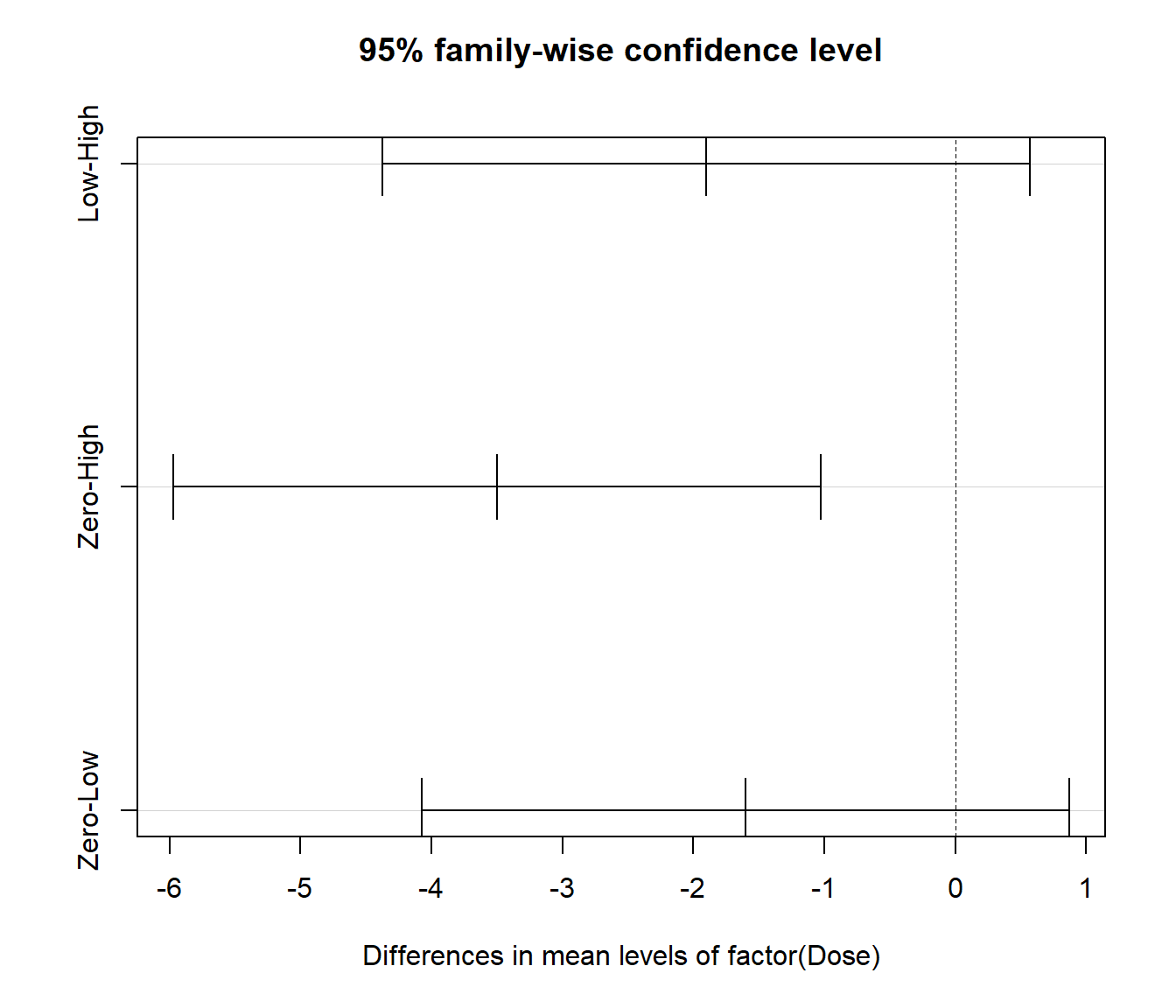
Low-High  -1.9 -4.371139  0.5711391 0.1562593
Zero-High -3.5 -5.971139 -1.0288609 0.0043753
Zero-Low  -1.6 -4.071139  0.8711391 0.2606999
The CIs and p-value show only one pair of means have a significant difference. The plot is optional and just helps us visualise the results: if the CI includes zero then the means are not significantly different.
20.3.6 Dunnett intervals
Dunnett intervals use a different multiplier because they just compare each group to a control level. So for the Caffeine analysis that is just two comparisons instead of three. The benefit of Dunnett intervals is narrower intervals than for Tukey, since we don’t have to adjust for so many chance ‘significant’ results. To use it, one needs to load the package DescTools.
  Dunnett's test for comparing several treatments with a control :
    95% family-wise confidence level

$Zero
          diff     lwr.ci   upr.ci   pval
High-Zero  3.5  1.1741746 5.825825 0.0030 **
Low-Zero   1.6 -0.7258254 3.925825 0.2065

---
Signif. codes:  0 '***' 0.001 '**' 0.01 '*' 0.05 '.' 0.1 ' ' 1
20.3.7 Discussion
Post hoc multiple comparisons are problematic, both in terms of the interpretation of test results and how they control for type I error (the significant level).
The type I error problem can be partially resolved by using arbitrary adjustment of the significance level of each test (e.g. Bonferroni adjustment \(\alpha/ \frac{K(K-1)}{2}\)) or some other adjustment of the multiplier.
The problem of interpretation of test results is more difficult. In the end some statisticians feel that multiple post hoc comparisons are often best avoided, and advocate simply inspecting parameter estimates as typically a good way to examine the inter-group differences. However one must remember that conclusions may need to be “taken with a grain of salt”.
20.1.1 Comments on the Diagnostic Plots
For a factor model, the fitted values are constant within each group. This explains the vertical lines in the left-hand plots.
A balanced factor design exists when the same number of observations are taken at each factor level.
When the data are balanced the leverage is constant, so a plot of the leverage would be pointless.
As a result, R produces a plot of standardized residuals against factor levels for balanced factor models in place of the usual residuals versus leverage plot.
For factor models, it is particularly important to scrutinize the plots for heteroscedasticity (non-constant variance), when the error variance changes markedly between the factor levels.
When heteroscedasticity is present, assumption A3 fails and conclusions based on F tests become unreliable.
The diagnostic plots do not provide any reason to doubt the appropriateness of the fitted model.