Lecture 5 Checking the Assumptions
Statistical models allow us to answer questions using data.
The validity of the conclusions that we reach is contingent upon the appropriateness of the models that we use.
Once you have fitted a statistical model to data, it is therefore important to check the assumptions underlying the model.
The tools to check these assumptions are often referred to as model diagnostics.
We shall look at assumption checking for simple linear regression in this lecture.
5.1 Assumptions for Simple Linear Regression
Recall that the linear regression model is \[Y_i = \beta_0 + \beta_1 x_i + \varepsilon_i\]
where we make the following assumptions:
A1. \(E[\varepsilon_i] = 0\) for i=1, … ,n.
A2. \(\varepsilon_1, \ldots ,\varepsilon_n\) are independent.
A3. var\((\varepsilon_i) = \sigma^2\) for i=1,…,n (homoscedasticity).
A4. \(\varepsilon_1, \ldots ,\varepsilon_n\) are normally distributed.
Class Discussion: Interpret these assumptions, and think about situations in which each might fail.
5.2 Raw Residuals
The residuals (or raw residuals), \[\begin{aligned} e_i &=& y_i - \hat \mu_i\\ &=& y_i - \hat \beta_0 - \hat \beta_1 x_i~~~~~~~~~(i=1,\ldots ,n)\end{aligned}\] are a fundamental diagnostic aid.
These residuals are a kind of sample version of the error random variables \(\varepsilon_1,\ldots,\varepsilon_n\).
Consequently we can test the assumptions by seeing if they hold for \(e_1, \ldots ,e_n\) (instead of \(\varepsilon_1, \ldots ,\varepsilon_n\)).
5.3 Standardized Residuals
There is a technical problem with raw residuals as substitutes for the error terms: it can be shown that the variance of the ith raw residual is given by \[var(e_i) = \sigma^2 (1 - h_{ii})~~~~~~(i=1,\ldots,n)\] where \[h_{ii} = \frac{1}{n} + \frac{(x_i - \bar x)^2}{s_{xx}}.\]
Hence unlike error terms, raw residuals do not have equal variance.
It is therefore preferable to work with the standardized residuals, defined by \[r_i = \frac{e_i}{s \sqrt{1-h_{ii}}}.\]
We will not need to evaluate this formula; R can produce standardized residuals for us.
These standardized residuals have an approximately standard normal, N(0,1), distribution and thus common variance.
In reality this technical issue is not a biggie. In practice there is little visual difference between looking at a graph of ordinary residuals and a graph of standardized residuals. For example the following plots show ordinary and standardized residuals for the Hill data introduced below. It is very hard to pick any difference in the shape of the points.
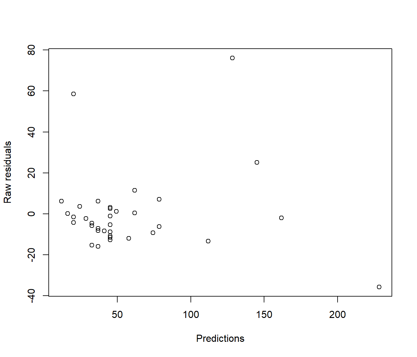
(#fig:Comparing residual plots-1)Plots of raw (upper) and standardised (lower) residuals against the predictions from the simple model.
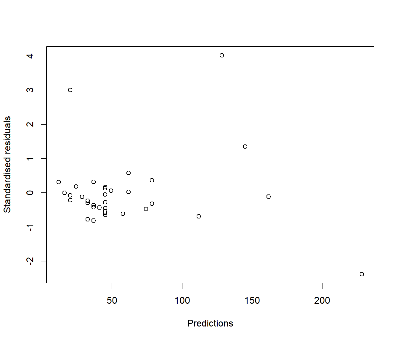
(#fig:Comparing residual plots-2)Plots of raw (upper) and standardised (lower) residuals against the predictions from the simple model.
5.3.1 So why do we bother with standardised residuals?
A practical reason is interpretability.
- If the units in which y is measured are very interpretable (such as $, or kg) then the same units apply to the raw residuals, and so the graph will be more interpretable in the original units.
- But suppose the units in which y is measured is rather arbitrary, such as the total from a certain number of questions on a questionnaire used to investigate some opinion, with each question being recorded on some arbitrary scale (e.g. 1=strongly disagree, 2=disagree, 3=neutral, 4=agree, 5 =strongly agree). In that case the precise values of y are not informative. E.g. if you were told your political score was 32, what does that mean? It would only have meaning if you knew what the average, and maximum and minimum attainable score were. So it is better to convert y to a z-score so that the numbers become more interpretable.
\[ z = \frac{y - \bar{y}}{s_y}\]
E.g. we can interpret z=0 as average, -2 as very low, z=+1 as above average, etc.
- Similarly the raw residuals will have the same uninterpretable units as y, but we can interpret standardised residuals as z-scores. \(r_i=-2\) meaning the \(y_i\) value is far below the regression line, \(r_i=0\) as meaning the \(y_i\) value is on the regression line, and \(r_i= +2.5\) meaning the \(y_i\) value is unusually far above the regression line, etc.
5.4 Scottish Hill Racing Data
- Data comprise the record times in 1984 for 35 Scottish hill races.
Variables are dist distance (miles) climb height gained (ft) time record time (minutes)
- Data source: A.C. Atkinson (1986) Comment: Aspects of diagnostic regression analysis. Statistical Science 1, pp397-402.

Figure 5.1: a hill runner
We will first consider simple linear regression of time on dist in R.
Reading the Data into R
data(hills, package = "MASS")
Hills <- hills
## Hills <- read.csv(file = "https://r-resources.massey.ac.nz/data/161251/hills.csv",
##     header = TRUE, row.names = 1)
The row.names=1 argument tells R that the first column of data in the comma separated values file hills.csv contains information which should provide the row names for the data (in this case, names of race locations).
The data is also available in the MASS package that comes with R. (Use one of these two data sources, not both!)
5.4.1 Fitting the Regression Model in R
Call:
lm(formula = time ~ dist, data = Hills)

Residuals:
    Min      1Q  Median      3Q     Max
-35.745  -9.037  -4.201   2.849  76.170

Coefficients:
            Estimate Std. Error t value Pr(>|t|)
(Intercept)  -4.8407     5.7562  -0.841    0.406
dist          8.3305     0.6196  13.446 6.08e-15 ***
---
Signif. codes:  0 '***' 0.001 '**' 0.01 '*' 0.05 '.' 0.1 ' ' 1

Residual standard error: 19.96 on 33 degrees of freedom
Multiple R-squared:  0.8456,    Adjusted R-squared:  0.841
F-statistic: 180.8 on 1 and 33 DF, p-value: 6.084e-15library(ggplot2)
ggplot(Hills, mapping = aes(y = time, x = dist)) + geom_point() + geom_smooth(method = "lm",
se = FALSE) + ylab("Winning time of race") + xlab("Race distance")`geom_smooth()` using formula = 'y ~ x'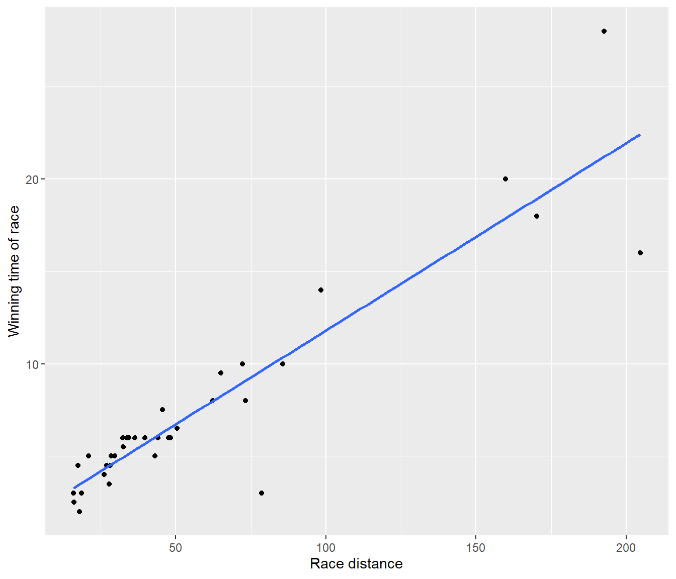
Figure 5.2: Fitted line plot for the first model for the hill racing data
The fitted model is (to 2 decimal places)
\[E[\mbox{time}] = -4.84 + 8.33 \, \mbox{dist}\]
The P-value of \(6.083904\times 10^{-15}\) for testing whether the regression slope is zero. This is tiny, and indicates overwhelming evidence for (linear) dependence of race time on distance.
The R-squared statistic of 0.8456 indicates that distance explains quite a large proportion of the variation in race record times.
The command resid() returns (raw) residuals for a fitted linear regression model.
     Greenmantle         Carnethy     Craig Dunain          Ben Rha
      0.09757971       3.20798304     -11.49201696     -12.03770125
      Ben Lomond         Goatfell     Bens of Jura      Cairnpapple
      0.46407065      11.41407065      76.17042112      -8.77501696
          Scolty         Traprain      Lairig Ghru           Dollar
     -7.06156077      -5.39201696     -35.74505318       6.23843923
         Lomonds      Cairn Table       Eildon Two        Cairngorm
     -9.29861363      -1.00901696      -5.71333268      -6.21384173
     Seven Hills       Knock Hill       Black Hill       Creag Beag
    -13.36866650      58.49935161     -15.22933268      -8.40978887
    Kildcon Hill Meall Ant-Suidhe   Half Ben Nevis         Cow Hill
     -4.20064839       3.58412351       2.49098304       6.11280780
   N Berwick Law       Creag Dubh        Burnswark        Largo Law
     -1.46764839      -2.26410458     -10.70901696      -8.24456077
         Criffel           Acmony        Ben Nevis      Knockfarrel
      1.19275494     -15.86156077       7.11915827     -12.75901696
   Two Breweries        Cockleroi     Moffat Chase
     25.14250874      -4.54633268      -1.93540365
These numbers are interpretable because the numbers are in units of minutes above or below what would be expected.
Let’s see the commands used to get those graphs of raw and standardised residuals shown earlier.
data(hills, package = "MASS")
Hills <- hills
Hills.lm = lm(time ~ dist, data = Hills)
plot(resid(Hills.lm) ~ predict.lm(Hills.lm), xlab = "Predictions", ylab = "Raw residuals")
Figure 5.3: Plots of raw (upper) and standardised (lower) residuals against the predictions from the simple model.
plot(rstandard(Hills.lm) ~ predict.lm(Hills.lm), xlab = "Predictions", ylab = "Standardised residuals")
Figure 5.4: Plots of raw (upper) and standardised (lower) residuals against the predictions from the simple model.
and some numerical details:
   Min. 1st Qu.  Median    Mean 3rd Qu.    Max.
-35.745 -9.037 -4.201 0.000 2.849 76.170 Min. 1st Qu. Median Mean 3rd Qu. Max.
-2.377778 -0.460171 -0.215778 -0.009795 0.145043 4.018411 5.5 Diagnostics for Failure of Model Assumptions
5.5.1 Assessing Assumption A1
Assumption A1 is equivalent to stating \(E[Y_i] = \beta_0 + \beta_1 x_i\)
Failure of A1 indicates that we are fitting the wrong mean function.
Looking for any trends in residual versus fitted values or a covariate is a useful diagnostic.
5.5.2 Assessing Assumption A2
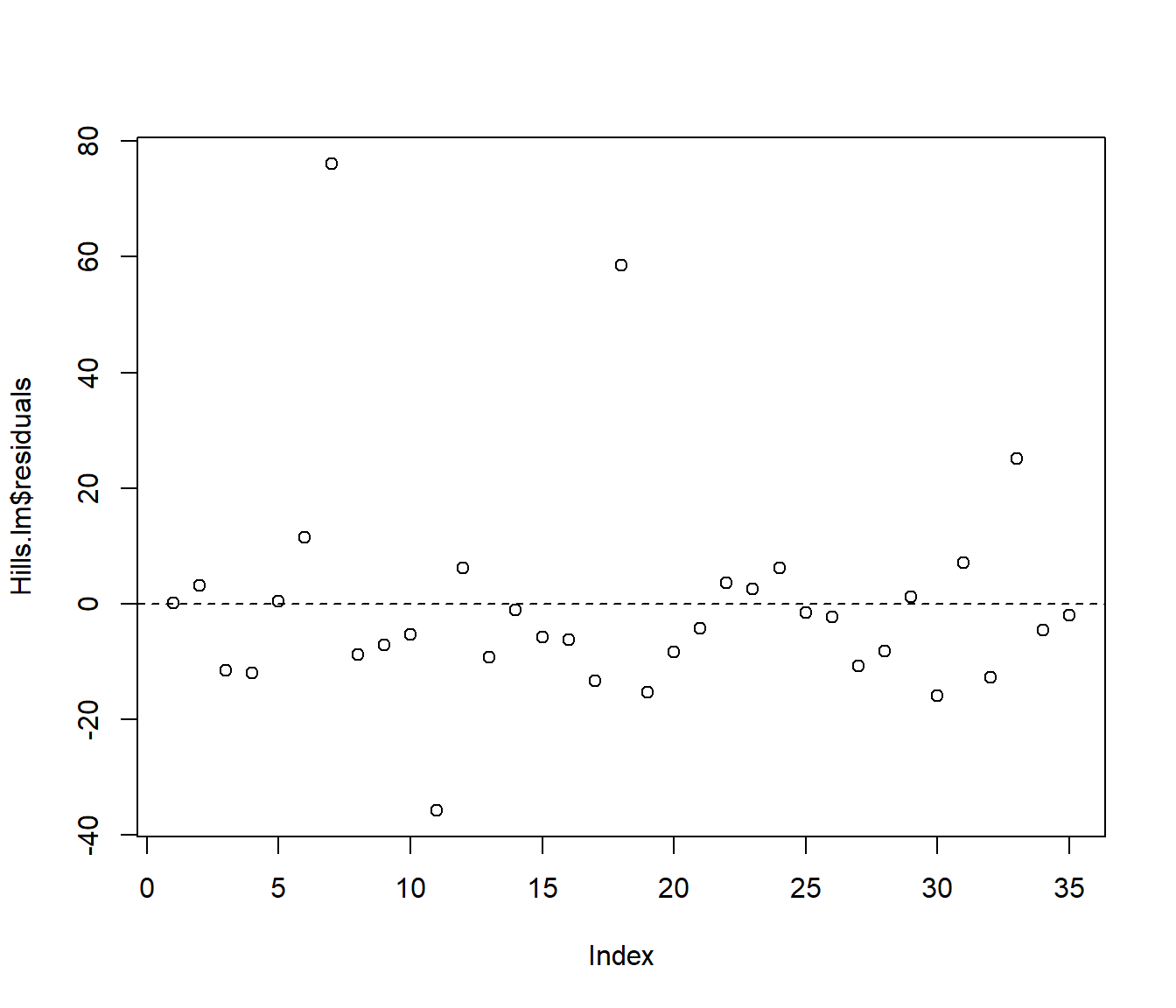
If A2 is correct, then residuals should appear randomly scattered about zero if plotted against race order (if known), fitted values or the predictor.
Long sequences of positive residuals followed by sequences of negative residuals suggests that the error terms are not independent.
Failure of this assumption will mean standard errors will be incorrect, and so hypothesis tests and confidence intervals will be unreliable.
We will look at regression models for time series later in the course.
5.5.3 Assessing Assumption A3
If A3 is correct, then the spread of the (standardized) residuals about zero should not vary systematically with the fitted value or covariate.
Heteroscedasticity (unequal spread) is typically recognized as a “fanning out” of (standardized) residuals when plotted against fitted value or covariate. This means the errorvariance increases with the mean response. (Alternatively one could have fanning in).
Failure of this assumption will leave parameter estimates unbiased, but standard errors will be incorrect, and hence test results and confidence intervals will be unreliable.
A transformation of both response and predictor variables can sometimes help in this case.
An alternative strategy is to use weighted linear regression (covered later in the course).
5.5.4 Assessing Assumption A4
A normal probability plot, or normal Q-Q plot, is a standard graphical tool for assessing the normality of a data set.
A normal Q-Q plot of the (standardized) residuals should show points staying close to a straight line — curvature indicates a failure of A4.
On the other hand failure of the normality assumption for the error distribution is not usually a serious problem. Removal of (obvious) outliers will often improve the normality of the standardized residuals.
5.6 Diagnostics for Hill race s Example
The plot() command applied to the fitted model Hills.lm produces four useful diagnostic plots. The par() command put first splits the graphing window into a two-by-two grid so we can see all four graphs together.
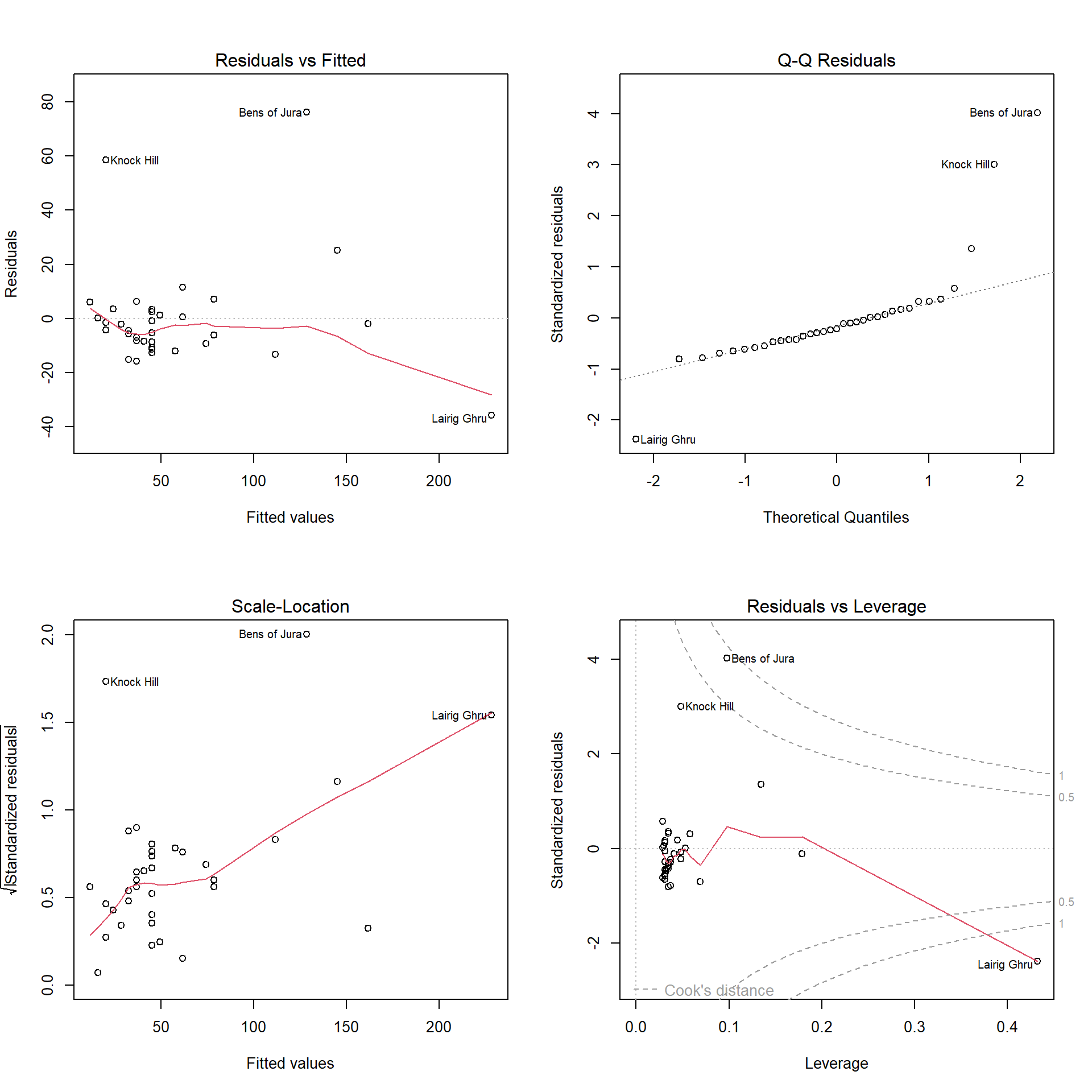
(#fig:Hills.lmDiag)Residual analysis plots for the first model applied to the hill racing data.
The first three of these plots are:
- Plot of raw residuals versus fitted values
- Normal Q-Q plot for standardized residuals
- Scale-location plot (square root of absolute standardized residuals against fitted value)
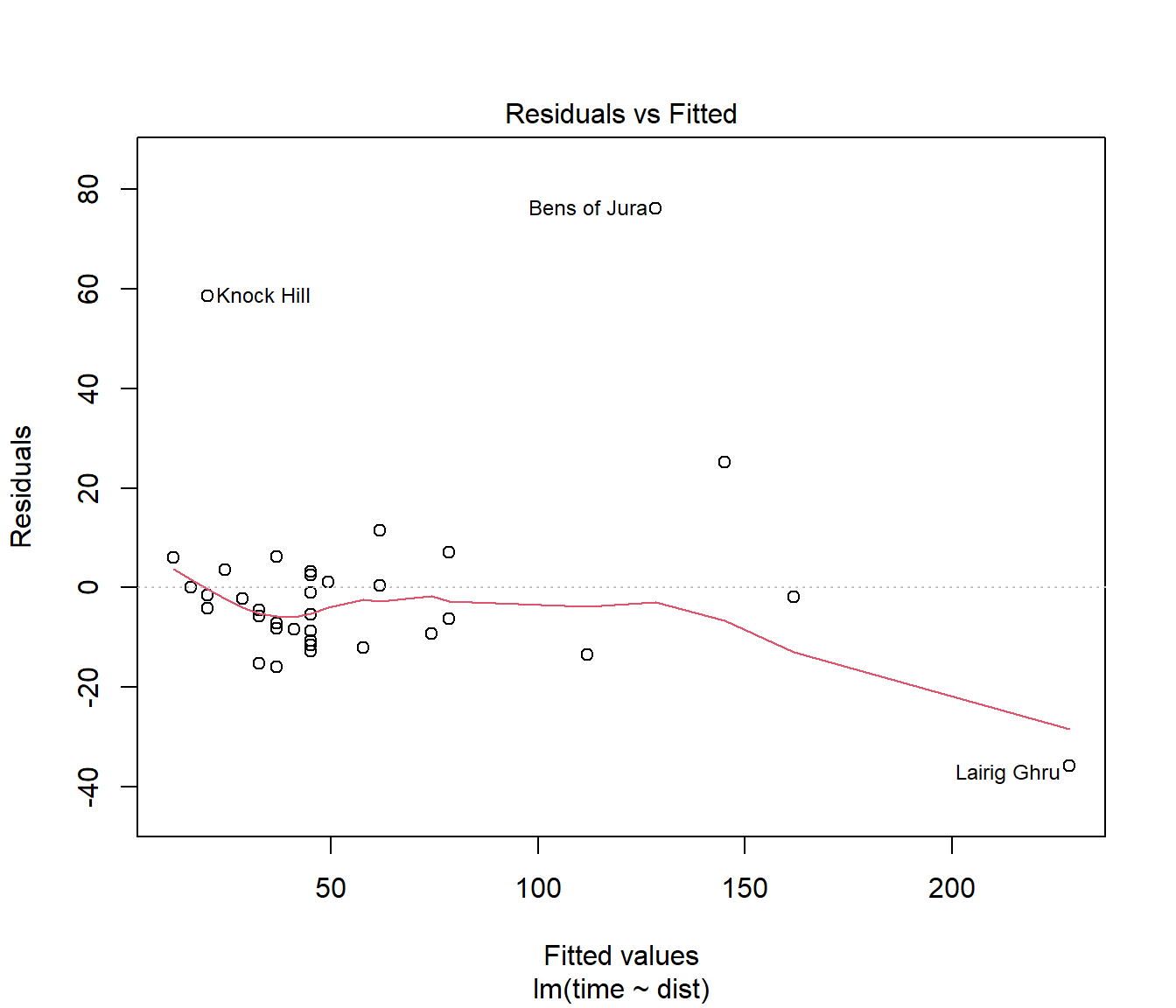
(#fig:Hills.lmDiag1)Residuals plotted against fitted values for the first model fitted to the hill racing data
This residual plot shows some data points with very large residuals.
The red line is a nonparametric estimate of trend (take care not to over-interpret) it.
Would you say there is strong evidence of curvature, or of increasing spread in residuals?
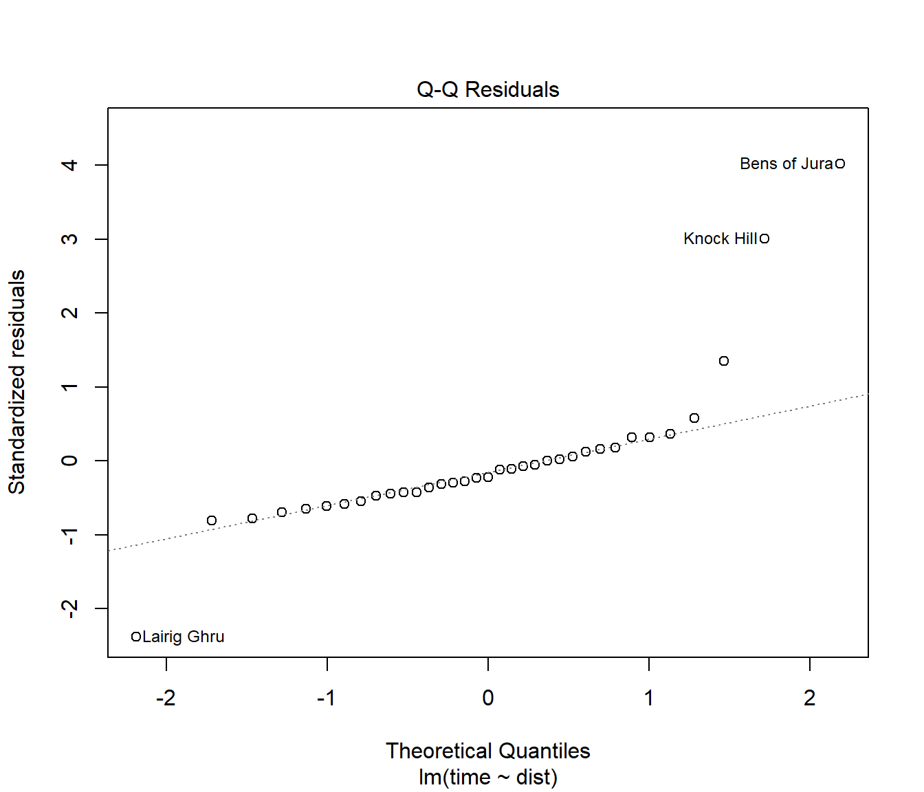
(#fig:Hills.lmDiag2)Normality plot of residuals for the first model fitted to the hill racing data
The Normal Q-Q plot is far from a straight line. This indicates failure of the normality assumption.
Note that this plot is heavily influenced by data points with large residuals.
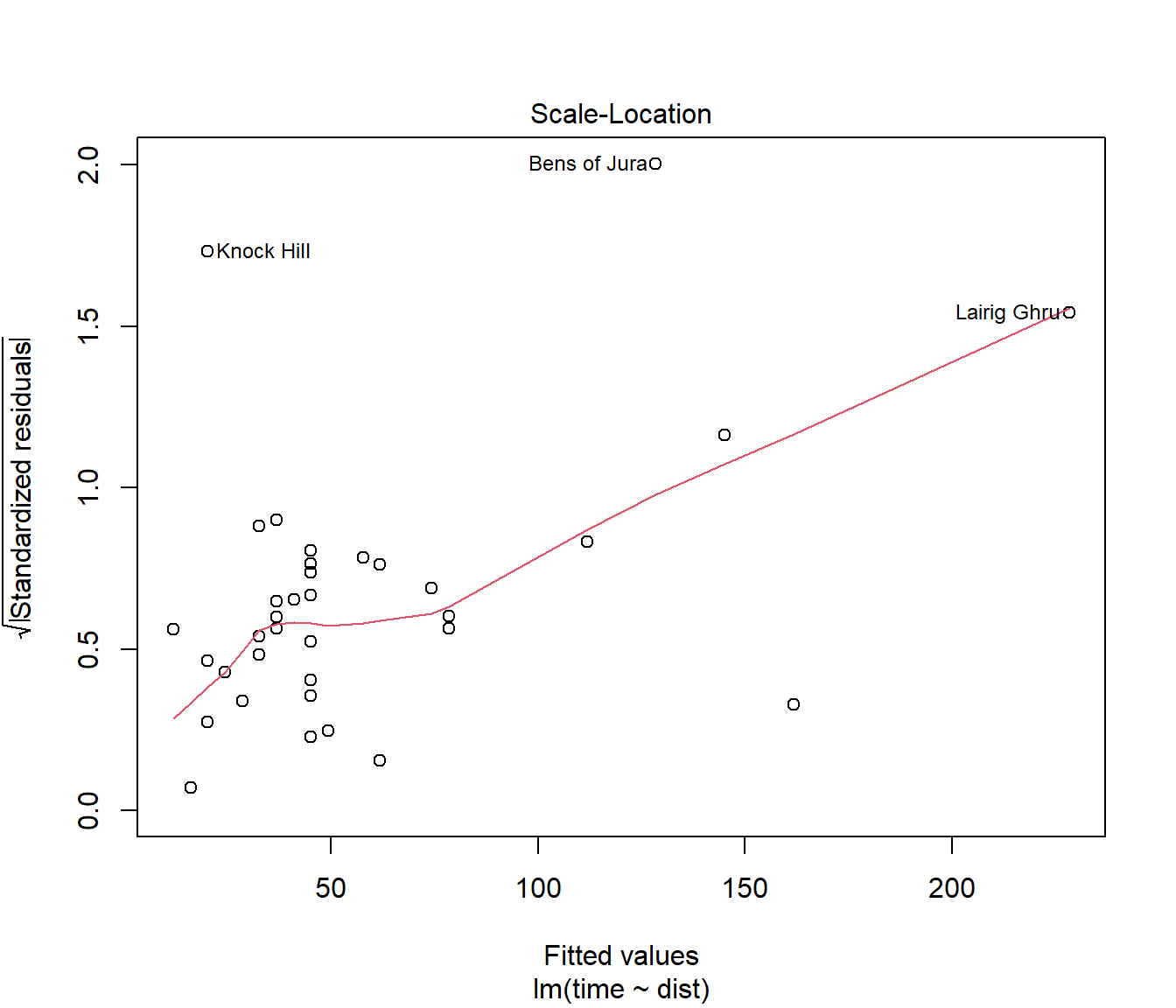
(#fig:Hills.lmDiag3)Scale versus location plot for the first model fitted to the hill racing data
For the scale-location plot, we look for a trend for the line to be increasing (or decreasing) as we move from left to right. If so, it provides a hint that spread of residuals is increasing (or decreasing) with fitted value.
This graph suggests the error variance \(\sigma^2\) may not be constant for all data points.
5.7 Conclusions from Diagnostics for Example
Linear regression model assumptions do not appear valid.
Hence conclusions based on this model are questionable.
Problems with model seem largely down to a few odd data points or outliers.
5.8 Practical Exercises
You should now be able to make a good start on this week’s practical exercises. See the first one and the second one