Lecture 16 Polynomial Regression Models
Simple and multiple regression models are types of linear model.
Remember that the word linear refers to the fact that the response is linearly related to the regression parameters, not to the predictors.
In most regression models, the relationship between the response and each of the explanatory variables is linear.
We can represent more general relationships using polynomial functions of the explanatory variables.
The resulting models are often referred to as polynomial regression models.
16.1 Child Lung Function Data
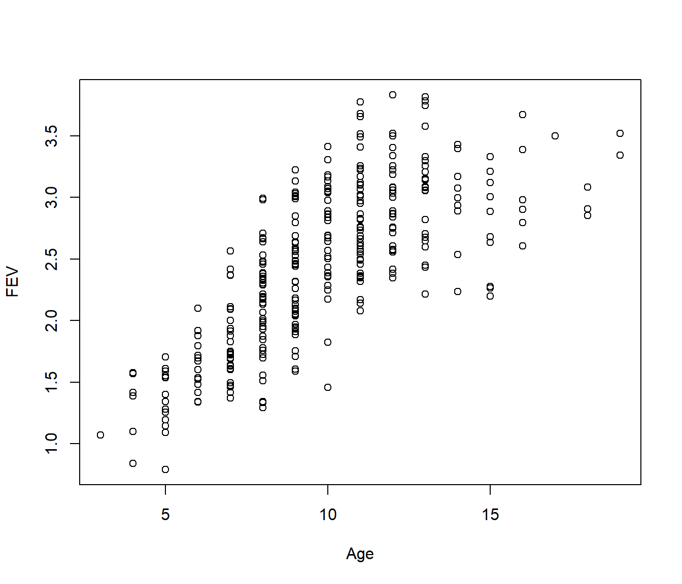
FEV (forced expiratory volume) is a measure of lung function. The data include determinations of FEV on 318 female children who were seen in a childhood respiratory disease study in Massachusetts in the U.S. Child’s age (in years) also recorded. Of interest to model FEV (response) as function of age.
Data source: Tager, I. B., Weiss, S. T., Rosner, B., and Speizer, F. E. (1979). Effect of parental cigarette smoking on pulmonary function in children. American Journal of Epidemiology, 110, 15-26.
16.2 The Polynomial Regression Model
The polynomial linear regression model is \[Y_i = \beta_0 + \beta_1 x_{i} + \beta_2 x_i^2 + \ldots + \beta_p x_{i}^p + \varepsilon_i ~~~~~~~~~ (i=1,\ldots,n)\]
where \(Y_i\) and \(x_i\) are the response and explanatory variable observed on the \(i\)th individual.
\(\varepsilon_1, \ldots \varepsilon_n\) are random errors satisfying the usual assumptions A1 to A4.
\(\beta_0, \beta_1, \ldots, \beta_p\) are the regression parameters.
The polynomial regression equation and A1 imply that \[E[Y_i] = \mu_i = \beta_0 + \beta_1 x_{i} + \beta_2 x_i^2 + \ldots + \beta_p x_{i}^p\]
The reasoning behind adding powers of the predictor (\(x_i^2, x_i^3\), etc) in the model is that the resulting relationship between the predictor variable and the response is no longer a line but rather a curve. Adding higher power terms results in more complex shapes.
16.3 Notes on The Polynomial Regression Model
We have defined a pth order polynomial regression model.
- Typically statisticians aim for low order polynomial models
- having p larger than 5 or 6 is unusual.
- If you use a polynomial model of order p, then you should include all terms of lower order (unless the circumstances are exceptional).
This last point is important. As an example, a cubic polynomial should include linear and quadratic terms: \[E[Y_i] = \beta_0 + \beta_1 x_{i} + \beta_2 x_i^2 + \beta_3 x_{i}^3\] is correct; we should not omit (e.g.) the quadratic term: \[E[Y_i] = \beta_0 + \beta_1 x_{i} + \beta_3 x_{i}^3\]
16.4 Example : Model Fitting in R
A sixth order polynomial model can be fitted with
Notice that the powers of Age appear within the function I(). This function “protects” its contents, in the sense that R reads the
contents as a normal mathematical expression.
For example, I(Age^4) is telling R to include the fourth power of Age in the
model.
N.B. the expressions *, / and ^ have a different meaning in
a model formula (explained in later lectures)
Modern practice is to avoid all that typing though!
16.4.1 Example : Sixth Order Model
Let’s start by trying to fit a sixth order model on the FEV data:
Call:
lm(formula = FEV ~ poly(Age, 6, raw = TRUE), data = Fev)

Residuals:
    Min      1Q  Median      3Q     Max
-1.2047 -0.2791  0.0186  0.2509  0.9210

Coefficients:
                            Estimate Std. Error t value Pr(>|t|)
(Intercept)               -1.520e+00  5.052e+00  -0.301    0.764
poly(Age, 6, raw = TRUE)1  2.079e+00  3.533e+00   0.588    0.557
poly(Age, 6, raw = TRUE)2 -6.468e-01  9.735e-01  -0.664    0.507
poly(Age, 6, raw = TRUE)3  1.033e-01  1.359e-01   0.761    0.447
poly(Age, 6, raw = TRUE)4 -8.145e-03  1.017e-02  -0.801    0.424
poly(Age, 6, raw = TRUE)5  3.056e-04  3.882e-04   0.787    0.432
poly(Age, 6, raw = TRUE)6 -4.360e-06  5.931e-06  -0.735    0.463

Residual standard error: 0.3902 on 311 degrees of freedom
Multiple R-squared:  0.6418,    Adjusted R-squared:  0.6349
F-statistic: 92.87 on 6 and 311 DF,  p-value: < 2.2e-16
The coefficient of poly(Age, 6) is not significant, so we can remove the 6th order term.
16.4.2 Example : Fifth Order Model
We now fit a fifth order polynomial model:
Call:
lm(formula = FEV ~ poly(Age, 5, raw = TRUE), data = Fev)

Residuals:
     Min       1Q   Median       3Q      Max
-1.19431 -0.27623  0.02088  0.24471  0.93266

Coefficients:
                            Estimate Std. Error t value Pr(>|t|)
(Intercept)                1.750e+00  2.393e+00   0.731    0.465
poly(Age, 5, raw = TRUE)1 -3.209e-01  1.349e+00  -0.238    0.812
poly(Age, 5, raw = TRUE)2  3.714e-02  2.858e-01   0.130    0.897
poly(Age, 5, raw = TRUE)3  5.707e-03  2.860e-02   0.200    0.842
poly(Age, 5, raw = TRUE)4 -7.392e-04  1.359e-03  -0.544    0.587
poly(Age, 5, raw = TRUE)5  2.083e-05  2.467e-05   0.844    0.399

Residual standard error: 0.3899 on 312 degrees of freedom
Multiple R-squared:  0.6412,    Adjusted R-squared:  0.6354
F-statistic: 111.5 on 5 and 312 DF,  p-value: < 2.2e-16
As the coefficient of poly(Age, 5) is not significant, we can remove the 5th order term from the model.
16.4.3 Example : Fourth Order Model
We now try a fourth order polynomial model:
Call:
lm(formula = FEV ~ poly(Age, 4, raw = TRUE), data = Fev)

Residuals:
     Min       1Q   Median       3Q      Max
-1.20203 -0.27466  0.02218  0.24525  0.93709

Coefficients:
                            Estimate Std. Error t value Pr(>|t|)
(Intercept)                3.5685906  1.0434415   3.420 0.000709 ***
poly(Age, 4, raw = TRUE)1 -1.3941151  0.4529027  -3.078 0.002267 **
poly(Age, 4, raw = TRUE)2  0.2712825  0.0692350   3.918 0.000110 ***
poly(Age, 4, raw = TRUE)3 -0.0181507  0.0044318  -4.096 5.37e-05 ***
poly(Age, 4, raw = TRUE)4  0.0004055  0.0001007   4.029 7.05e-05 ***
---
Signif. codes:  0 '***' 0.001 '**' 0.01 '*' 0.05 '.' 0.1 ' ' 1

Residual standard error: 0.3897 on 313 degrees of freedom
Multiple R-squared:  0.6404,    Adjusted R-squared:  0.6358
F-statistic: 139.3 on 4 and 313 DF,  p-value: < 2.2e-16
The fourth order term is statistically significant, so this is our preferred model. Since the 4th order term is significant, we have to keep all lower order terms.
Our fitted model equation is: \[E[\mbox{FEV}] = 3.57 - 1.39~\mbox{Age} + 0.27~\mbox{Age}^2 - 0.018~\mbox{Age}^3 + 0.00041~\mbox{Age}^4\]
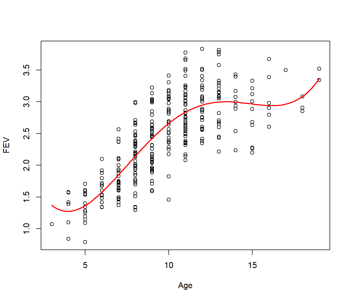
Looking at the plot (above), the fitted model looks adequate for ages in the range 5 to 15 years. At the extreme ends of the plot the fitted curve exhibits spurious upward curvature. This feature of the plot is an artifact of the form of the polynomial rather than a characteristic of the data.
16.4.4 Example : Collinearity in the Fitted Model
Notice how in the 6th and 5th order models, none of the regression coefficients are significant; however when dropping to a 4th order model this leads to significant t-statistics. This is due to a noticeable collinearity between the powers of Age.
Collinearity in polynomial regression can lead to numerical instability in statistical software packages.
Problems of collinearity can be addressed by using orthogonal polynomials, coming up in a lecture quite soon.
16.5 Numeric instability (??)
Successive powers of our predictor variable frequently end up being on very different orders of magnitude. Just for the sake of illustration, let’s use a predictor taking on values from ten to one-hundred in steps of ten.
[1] 10 20 30 40 50 60 70 80 90 100and take it out to the sixth power…
 [1] 1.00000e+06 6.40000e+07 7.29000e+08 4.09600e+09 1.56250e+10 4.66560e+10
 [7] 1.17649e+11 2.62144e+11 5.31441e+11 1.00000e+12
When these two vectors end up in the same model matrix, the magnitude of the largest value swamps the little numbers in the matrix when we are finding the inverse matrix \((X^t X)^{-1}\) when fitting the linear model.
We can avoid some of this problem by re-scaling the original x variable, by centering (subtract the mean), seen next lecture; we could then multiply by a scalar to bring the resulting values into the range -1 to 1, before using the powers (not shown in this course).
This re-scaling keeps the same information within the original x variable as it hasn’t changed shape or been re-ordered in any way. It’s like deciding to measure something in centimetres or re-scaling to metres; the true measurements won’t change, just their representation in numeric terms.