Lecture 9 Introduction to Multiple Linear Regression
This lecture will cover an introduction to regression with multiple explanatory variables.
9.1 Scottish Hill Racing Data Revisited
For the linear model of time against dist , plot residuals against climb .
data(hills, package = "MASS")
Hills.lm <- lm(time ~ dist, data = hills)
plot(resid(Hills.lm) ~ climb, data = hills, xlab = "Climb")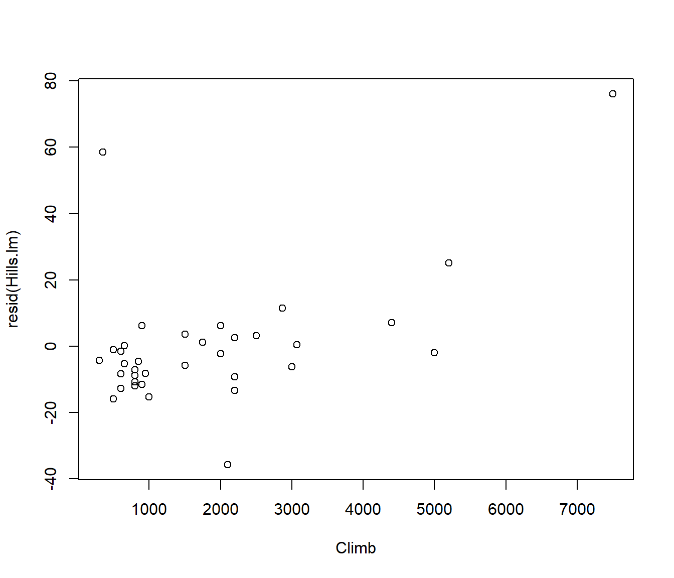
This is a lurking variable plot. That is, it shows that the residuals are correlated with another variable not in the model, implying that if we include that variable in the regression model it will explain more of the data.
For the Scottish Hill Racing data, the trend in the lurking variable plot of residuals against
climbindicates that the height climbed should be included in the model in addition to the race distance.For applications such as this we need to extend simple linear regression to incorporate multiple predictors.
This extended methodology is called multiple linear regression.
9.2 The Multiple Linear Regression Model
The multiple linear regression model is \[Y_i = \beta_0 + \beta_1 x_{i1} + \ldots + \beta_p x_{ip} + \varepsilon_i\] for i=1,2,…,n.
Note now that:
There are p predictor variables x1, x2, …, xp.
The notation xij denotes the value of xj for the ith individual.
\(\varepsilon_1, \ldots \varepsilon_n\) are random errors satisfying assumptions A1 — A4.
\(\beta_0, \beta_1, \ldots, \beta_p\) are the regression parameters.
9.3 Parameter Estimation
The equation for the regression line and A1 imply that \[E[Y_i] = \mu_i = \beta_0 + \beta_1 x_{i1} + \ldots + \beta_p x_{ip}\]
The parameters \(\beta_0,\beta_1, \ldots, \beta_p\) can be estimated by the method of least squares.
The least squares estimates (LSEs) \(\hat \beta_0,\hat \beta_1, \ldots ,\hat \beta_p\) are still the values that minimize the following sum of squares: \[\begin{aligned} SS(\beta_0, \beta_1, \ldots , \beta_p) &=& \sum_{i=1}^n (y_i - \mu_i)^2\\ &=& \sum_{i=1}^n (y_i - \beta_0 - \beta_1 x_{i1} - \ldots - \beta_p x_{ip} )^2\end{aligned}\]
Software packages can quickly compute LSEs.
9.4 Fitted Values and Residuals
The definitions of a fitted value and a residual in multiple linear regression follow on naturally from simple linear regression.
The ith fitted value is \[\hat \mu_i = \hat \beta_0 + \hat \beta_1 x_{i1} + \ldots + \hat\beta_p x_{ip}\]
The ith residual is \(e_i = y_i - \hat \mu_i\).
The error variance, \(\sigma^2\), can be estimated (unbiasedly) by \[s^2 = \frac{1}{n-p-1} RSS\] where the residual sum of squares is \(RSS = \sum_{i=1}^n (y_i - \hat \mu_i)^2\).
9.5 New Zealand Climate Data Example
| Variable | Description |
|---|---|
Y= MnJlyTemp |
Mean July temperature (degrees Celsius) |
MnJanTemp |
Mean January temperature (degrees Celsius) |
Lat |
Degrees of latitude (south) |
Long |
Degrees of longitude (east) |
Rain |
Annual precipitation (mm) |
Sun |
Annual hours of sunshine |
Height |
Average height above sea level (in metres) |
Sea |
0 = no (inland) 1 = yes is coastal |
NorthIsland |
0 = no, 1= yes |
Suppose our aim is to find a model that explains the mean July Temperature in the different locations, in terms of the other variables. We will sometimes refer to this variable MnJlyTemp as y and the others as x1, x2, …, x8 respectively.
Note it does not matter that x7 = Sea and x8 = NorthIsland are just 0 - 1 variables. These coded variables are called indicator variables and are an extremely important aspect of regression models, so important that they feature heavily in the rest of the course. Look out for them.
Eg. the slope \(\beta_7\) will still represent a one-unit change, i.e. the difference between a non-Coastal (Sea=0) and Coastal (Sea=1) location.
Download Climate.csv to be able to run the examples below.
            Lat  Long MnJanTemp MnJlyTemp Rain  Sun Height Sea NorthIsland
Kaitaia    35.1 173.3      19.3      11.7 1418 2113     80   1           1
Kerikeri   35.2 174.0      18.9      10.8 1682 2004     73   1           1
Dargaville 36.0 173.8      18.6      10.7 1248 1956     20   1           1
Whangarei  35.7 174.3      19.7      11.0 1600 1925     29   1           1
Auckland   36.9 174.8      19.4      11.0 1185 2102     49   1           1
Tauranga 37.7 176.2 18.5 9.3 1349 2277 4 1 1par(mfrow = c(1, 2))
plot(Lat ~ Long, pch = 2 - Sea, data = Climate)
plot(-Lat ~ Long, pch = NorthIsland + 16, col = NorthIsland + 3, data = Climate)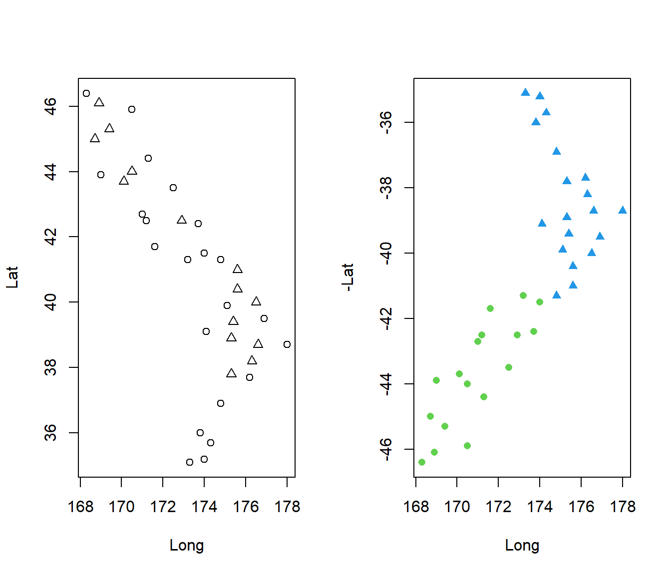
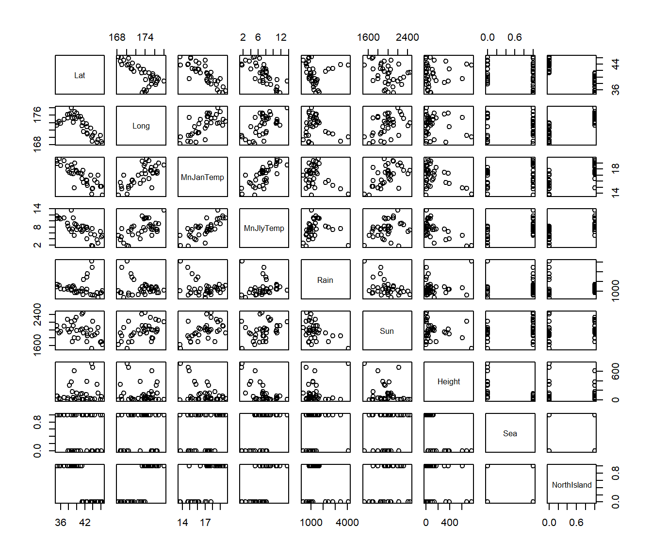
To get a quick overview of the data we can use the pairs() command to get a scatterplot matrix. Clearly the variables are related.
To fit a multiple regression \[E[Y_i] = \beta_0 + \beta_1 x_{i1} + \ldots + \beta_p x_{ip}\] you simply mention all the variables in the model statement of lm().
Climate.lm = lm(MnJlyTemp ~ MnJanTemp + Lat + Long + Rain + Sun + Height + Sea +
    NorthIsland, data = Climate)
summary(Climate.lm)
Call:
lm(formula = MnJlyTemp ~ MnJanTemp + Lat + Long + Rain + Sun +
    Height + Sea + NorthIsland, data = Climate)

Residuals:
    Min      1Q  Median      3Q     Max
-1.2213 -0.5257 -0.2620  0.3796  3.3033

Coefficients:
              Estimate Std. Error t value Pr(>|t|)
(Intercept)  5.2829167 24.0200695   0.220  0.82757
MnJanTemp   -0.0380083  0.2901840  -0.131  0.89676
Lat         -0.3655501  0.1638323  -2.231  0.03416 *
Long         0.1012667  0.1253184   0.808  0.42611
Rain         0.0002901  0.0002971   0.977  0.33744
Sun         -0.0006941  0.0011596  -0.599  0.55442
Height      -0.0049986  0.0014557  -3.434  0.00194 **
Sea          1.7298287  0.5472228   3.161  0.00386 **
NorthIsland  1.3589549  0.8087868   1.680  0.10445
---
Signif. codes:  0 '***' 0.001 '**' 0.01 '*' 0.05 '.' 0.1 ' ' 1

Residual standard error: 0.9627 on 27 degrees of freedom
Multiple R-squared:  0.9074,    Adjusted R-squared:   0.88
F-statistic: 33.09 on 8 and 27 DF,  p-value: 5.255e-12
The \(R^2\) is interpreted the same as before: 90.7% of the variation in the Y values (mean July temperatures) is explained by the predictors.
The residual mean square = S is still interpreted as the standard deviation of the residuals. That is, S= 0.9627 represents the typical variation of the raw data (actual Y) around the fitted values. Putting it another way, we expect about \(95\%\) of data to be within \(2S \approx 2\) degrees of the predicted mean July temperature.
The information about residuals at the start of the summary output shows that the maximum residual is 3.3, so that means there is a location which it 3.3 degrees warmer in July than would be predicted by the covariates.
Now if we look at the table of coefficients we see that only three variables have significant P-values: Lat, Height and Sea.
The other variables are not significant. So it looks as though one or more of them need to be removed from the regression.
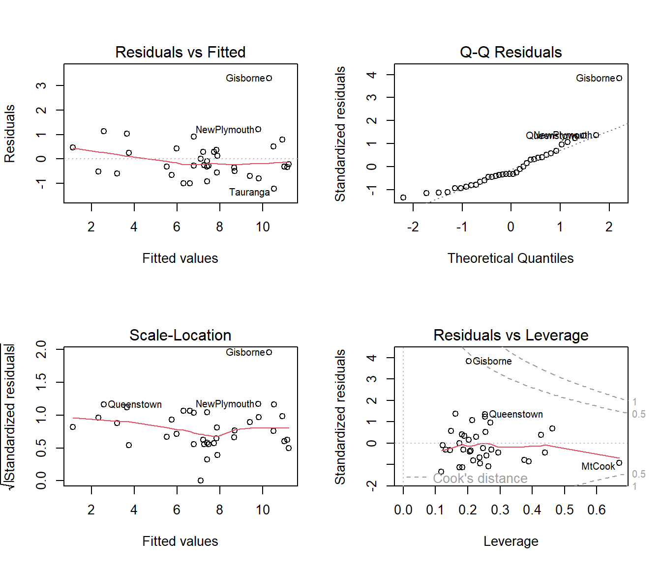
Looking at the residual plots, we see that row number 9 (Gisbourne, on the east coast of the North Island) is the location with the big residual. The first plot suggests a hint of curvature, but it is weak and it is too soon to worry about this when we need to remove some covariates.
from the normal Q-Q plot that, apart from row 9, the residuals are fairly normal, but row 9 has a standardized residual\(>3\). Many statistical programs automatically flag points with standardized residual\(>3\) as outliers.
The bottom right graph shows that row 9 is near the boundary for Cooks’ D > 0.5, but it is acceptable to say that no locations are having extraordinary influence on the regression coefficients. One location, row 28, is high leverage, which means its covariate values are unusual compared to those of other locations.
9.6 Adjusted \(R^2\) and F test
We will consider the F test in more detail later, but for now you should know that it looks to see whether there is anything in our model which is related to the response (Y) variable, whether that is a single variable or a group of variables. i.e. it tests the hypothesis that all the slopes are zero. \[H_0: \beta_1=\beta_2=...=\beta_p = 0\] If F is large we reject this hypothesis. For the moment we shall just consider the P-value. Since \(P= 5.255\times 10^{-12}\) this is an exceedingly small number, so we reject \(H_0\) and conclude that at least one of the slopes is non-zero.
The adjusted \(R^2\) is only used to compare two models with different numbers of regression parameters. When we add a variable to a regression model, the ordinary multiple \(R^2\) will go up, even if the variable added is rubbish. The adjusted \(R^2\) is an alternative formula which will only go up if the additional model explains more than at least one extra row of data. (This is a very weak criterion indeed).
Conversely if we delete a useless variable, the adjusted \(R^2\) should go up, or at least not go down.
Just for the sake of illustration, suppose we were to remove the variable with the biggest P-value in the previous regression, namely MnJanTemp, with a P-value of 0.897.
Call:
lm(formula = MnJlyTemp ~ Lat + Long + Rain + Sun + Height + Sea +
    NorthIsland, data = Climate)

Residuals:
    Min      1Q  Median      3Q     Max
-1.2167 -0.5622 -0.2556  0.3987  3.2860

Coefficients:
              Estimate Std. Error t value Pr(>|t|)
(Intercept)  4.0580828 21.7332488   0.187 0.853225
Lat         -0.3500826  0.1115481  -3.138 0.003978 **
Long         0.1011944  0.1230982   0.822 0.417987
Rain         0.0003045  0.0002712   1.123 0.270963
Sun         -0.0007389  0.0010886  -0.679 0.502865
Height      -0.0048888  0.0011689  -4.182 0.000257 ***
Sea          1.7495792  0.5167223   3.386 0.002118 **
NorthIsland  1.3678091  0.7916852   1.728 0.095055 .
---
Signif. codes:  0 '***' 0.001 '**' 0.01 '*' 0.05 '.' 0.1 ' ' 1

Residual standard error: 0.9456 on 28 degrees of freedom
Multiple R-squared:  0.9074,    Adjusted R-squared:  0.8842
F-statistic: 39.19 on 7 and 28 DF,  p-value: 8.063e-13
The adjusted \(R^2\) here is 0.8842. In the model with the extra variable MnJanTemp the adjusted \(R^2\) is 0.88. That is, if we were to add that variable back in to the model again then the adjusted \(R^2\) would go down. This is clear evidence that we do not need this variable MnJanTemp.
9.7 Simplifying the regression model
Clearly not all the variables in the ‘full’ regression model have significant p-values. (By ‘full’ model I mean with all the predictors X1,..,X8 in there). We need to find out which variables are in fact needed.
There are two main approaches to choosing a model
Forward selection, where we start from a likely one-variable model and build it up by adding in extra predictors one at a time.
Backwards elimination, where we start from a full model and drop non-significant variables out one at a time. This is usually the better method). We made a start at this by removing MnJanTemp from the big regression model. .
Since the predictors are usually not independent of each other, it is important to make any model changes one variable at a time. (We will see a reason for this later in the course).
Note we will study model selection techniques in more detail later on, where some automated procedures are introduced, including a hybrid forwards/backwards method called ’stepwise model selection’.
Before we get to that point, we will take the task slowly because we are aiming to understand what is going on.
We start by trying to use forward selection, beginning with the most highly correlated single variable.
               Lat   Long MnJanTemp MnJlyTemp   Rain    Sun Height    Sea
Lat          1.000 -0.754    -0.825    -0.763 -0.036 -0.367  0.136 -0.152
Long        -0.754  1.000     0.707     0.591 -0.231  0.459 -0.102 -0.020
MnJanTemp   -0.825  0.707     1.000     0.743 -0.304  0.556 -0.432  0.235
MnJlyTemp   -0.763  0.591     0.743     1.000  0.033  0.334 -0.613  0.577
Rain        -0.036 -0.231    -0.304     0.033  1.000 -0.440  0.198  0.097
Sun         -0.367  0.459     0.556     0.334 -0.440  1.000 -0.236  0.301
Height       0.136 -0.102    -0.432    -0.613  0.198 -0.236  1.000 -0.659
Sea         -0.152 -0.020     0.235     0.577  0.097  0.301 -0.659  1.000
NorthIsland -0.837  0.829     0.710     0.652 -0.125  0.242 -0.086 -0.070
            NorthIsland
Lat              -0.837
Long              0.829
MnJanTemp         0.710
MnJlyTemp         0.652
Rain             -0.125
Sun               0.242
Height           -0.086
Sea              -0.070
NorthIsland       1.000
Looking at the column for MnJlyTemp we see that the variables with biggest correlation are Lat (correlation = -0.763) and MnJanTemp (correlation = 0.743). Looking at the correlations would give us the same p-value as regressing the predictor by itself.
So why did the previous argument say that MnJanTemp was useless but now the correlations say it is highly related to y?
The answer is that virtually all of the information that MnJanTemp would bring to the regression, is already expressed in the other covariates. So by itself it is informative, but after everything else, MnJanTemp has nothing more to tell us about y = MnJlyTemp.
9.7.1 Single-Variable Model
We will start by regressing MnJlyTemp on Lat.
Call:
lm(formula = MnJlyTemp ~ Lat, data = Climate)

Residuals:
    Min      1Q  Median      3Q     Max
-3.6992 -0.9786  0.1566  1.0588  4.7930

Coefficients:
            Estimate Std. Error t value Pr(>|t|)
(Intercept) 34.42127    3.94299   8.730 3.35e-10 ***
Lat         -0.66187    0.09613  -6.885 6.25e-08 ***
---
Signif. codes:  0 '***' 0.001 '**' 0.01 '*' 0.05 '.' 0.1 ' ' 1

Residual standard error: 1.822 on 34 degrees of freedom
Multiple R-squared:  0.5824,    Adjusted R-squared:  0.5701
F-statistic: 47.41 on 1 and 34 DF,  p-value: 6.25e-08
Clearly Lat is significant.
Can you interpret the slope?
Can you interpret the intercept (is this realistic)? Hint: Think a bit about NZ’s location.
9.7.2 Trying a two-variable model
We will look to see what happens if we add in MnJanTemp or Height on top of the existing variable Lat.
Call:
lm(formula = MnJlyTemp ~ Lat + MnJanTemp, data = Climate)

Residuals:
    Min      1Q  Median      3Q     Max
-3.1955 -1.1055 -0.1844  1.3421  4.2562

Coefficients:
            Estimate Std. Error t value Pr(>|t|)
(Intercept)  13.6470    11.6982   1.167   0.2517
Lat          -0.4073     0.1643  -2.479   0.0184 *
MnJanTemp     0.6127     0.3263   1.878   0.0693 .
---
Signif. codes:  0 '***' 0.001 '**' 0.01 '*' 0.05 '.' 0.1 ' ' 1

Residual standard error: 1.758 on 33 degrees of freedom
Multiple R-squared:  0.6227,    Adjusted R-squared:  0.5998
F-statistic: 27.23 on 2 and 33 DF,  p-value: 1.037e-07
Call:
lm(formula = MnJlyTemp ~ Lat + Height, data = Climate)

Residuals:
    Min      1Q  Median      3Q     Max
-2.0607 -0.6215 -0.1021  0.5145  3.9898

Coefficients:
              Estimate Std. Error t value Pr(>|t|)
(Intercept) 32.8788366  2.4333203  13.512 5.30e-15 ***
Lat         -0.6005121  0.0596687 -10.064 1.38e-11 ***
Height      -0.0071984  0.0009542  -7.544 1.12e-08 ***
---
Signif. codes:  0 '***' 0.001 '**' 0.01 '*' 0.05 '.' 0.1 ' ' 1

Residual standard error: 1.121 on 33 degrees of freedom
Multiple R-squared:  0.8467,    Adjusted R-squared:  0.8374
F-statistic: 91.14 on 2 and 33 DF,  p-value: 3.639e-14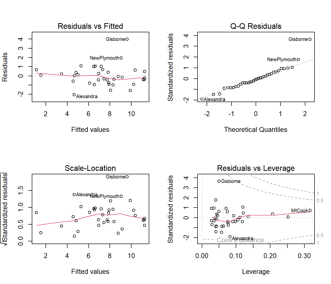
In the first analysis, MnJanTemp had a non-significant P-value, so again indicating that it is not useful. However the adjusted \(R^2\) does go up so we would not be able to dismiss it entirely.
In the second analysis Height is very significant and the adjusted \(R^2\) has gone up a very big amount, so it is right to include Height in the regression model.
However the diagnostic plots do not show much difference to the plots for the full model.
9.8 On regression diagnostics for multiple regression
When we had just one predictor on offer, we should have checked for nonlinearity in the relationship.
It is recommended before the multiple regression to plot Y vs each explanatory variable \(x_1, ..., x_p\) in turn to check for curvature.
But sometimes problems only show up once one has adjusted for other variables. So, after fitting the model plot residuals \(e_i\) against each \(x_i\), or use standardized residuals. Be boringly systematic.
And it’s a good idea to use a lowess smoother to check for possible curvature.
library(ggplot2)
Climate |>
    ggplot(aes(y = residuals(Climate.lm3), x = Height)) + geom_point() + geom_smooth()
`geom_smooth()` using method = 'loess' and formula = 'y ~ x'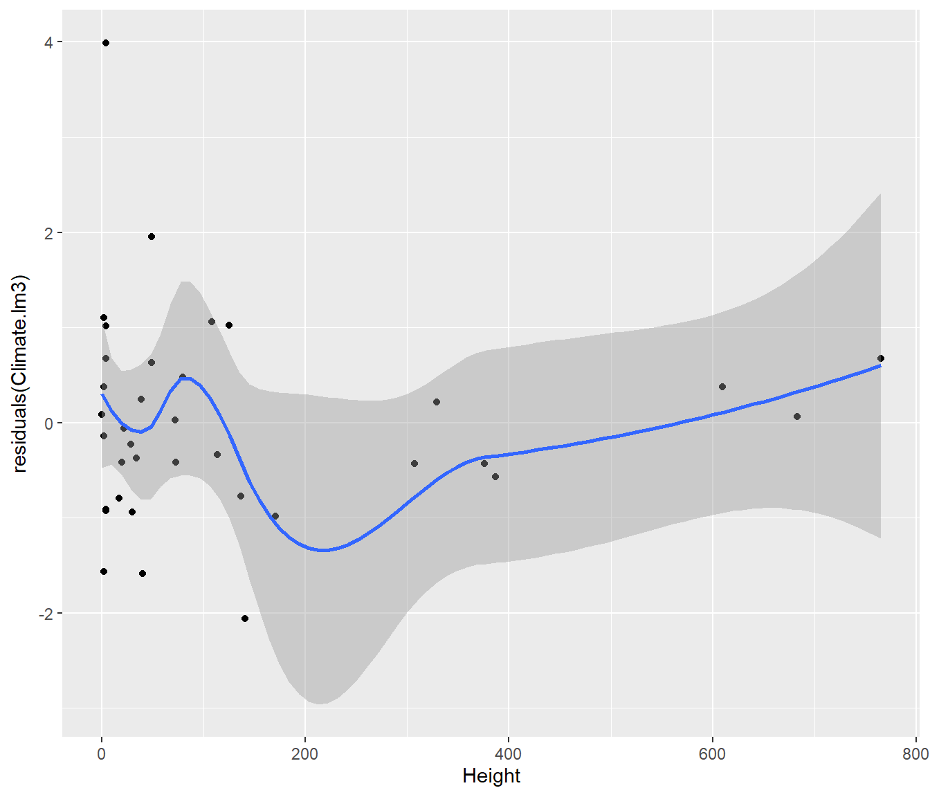
This graph shows possible curvature with height once latitude is allowed for: perhaps a transformation might give a better model? Something to think about later.
It is better to be alerted to a possible problem and be able to dismiss it, than to be unaware of the possible problem at all.
9.8.1 Outliers
Just as for the simple model, residuals are defined as \(e_i = y_i – \hat y_i\) .
And again, just as for the simple model, the standard errors for the residuals depends on how unusual the corresponding x values are. This complicates the interpretation of the graphs, so we can remove this complication by looking at standardized residuals which are scaled to give equal chance of spread at every x value. Standardized residuals should usually lie within the range \(\pm 2\), and very seldom \(<-3\) or \(> 3\)
Also as before, we can check for whether a particular point is dragging the line towards itself (and thus not appearing as unusual as it should) by computing externally studentized deleted residuals.
It is often helpful to plot the standardized and deleted residuals on the same graph, as that helps show whether the deletion is making a big difference.
plot(rstudent(Climate.lm3) ~ Climate.lm3$fitted.values, col = 2, pch = "+", main = "standardized(o) and studentized(+) residuals vs fitted values")
points(rstandard(Climate.lm3) ~ Climate.lm3$fitted.values)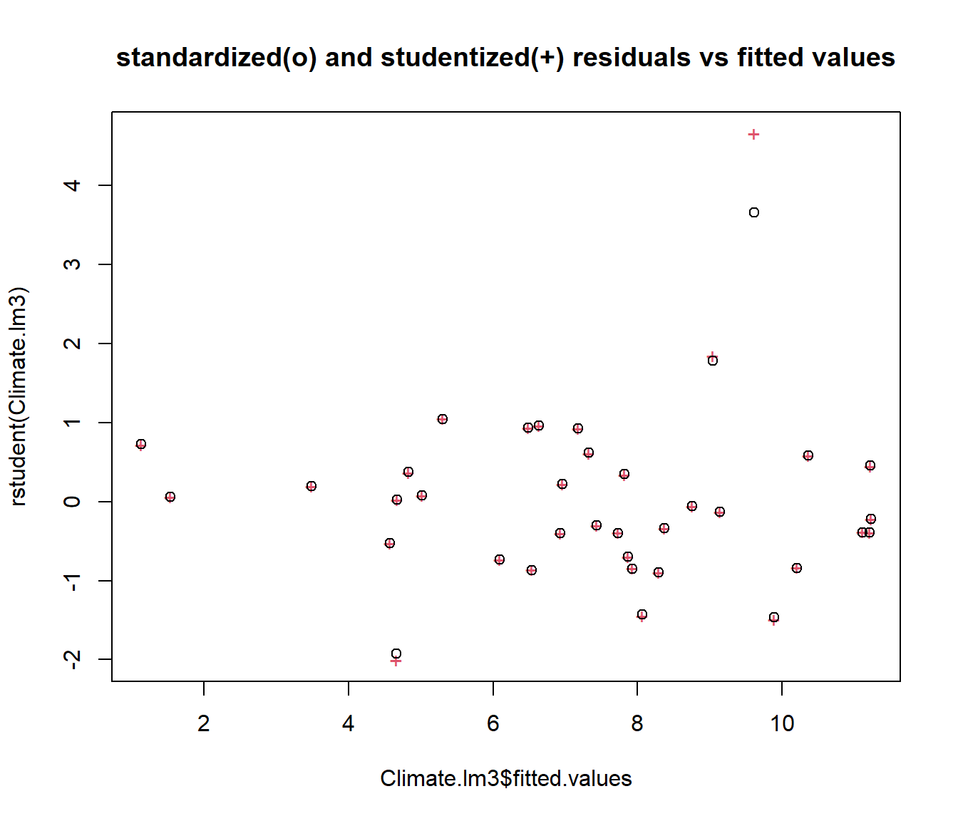
It is clear that deleting Gisborne would make a big difference to the regression, so we should check to make sure the number is correct. However deleting any other data points would make very little difference.
9.9 Checking leverage
The leverage values \(h_{ii}\) can be obtained using the hatvalues() function, and plotted against any variables of interest.
The average value of \(h_{ii}\) is \(p/n\).
Points with \(h_{ii} > 3 p/n\) are regarded as points worth checking.
For the Climate.lm3 model p=3 (intercept+ 2 slopes) and n=36.
plot(hatvalues(Climate.lm3) ~ Lat, data = Climate)
abline(h = 3 * length(coef(Climate.lm3))/nrow(Climate))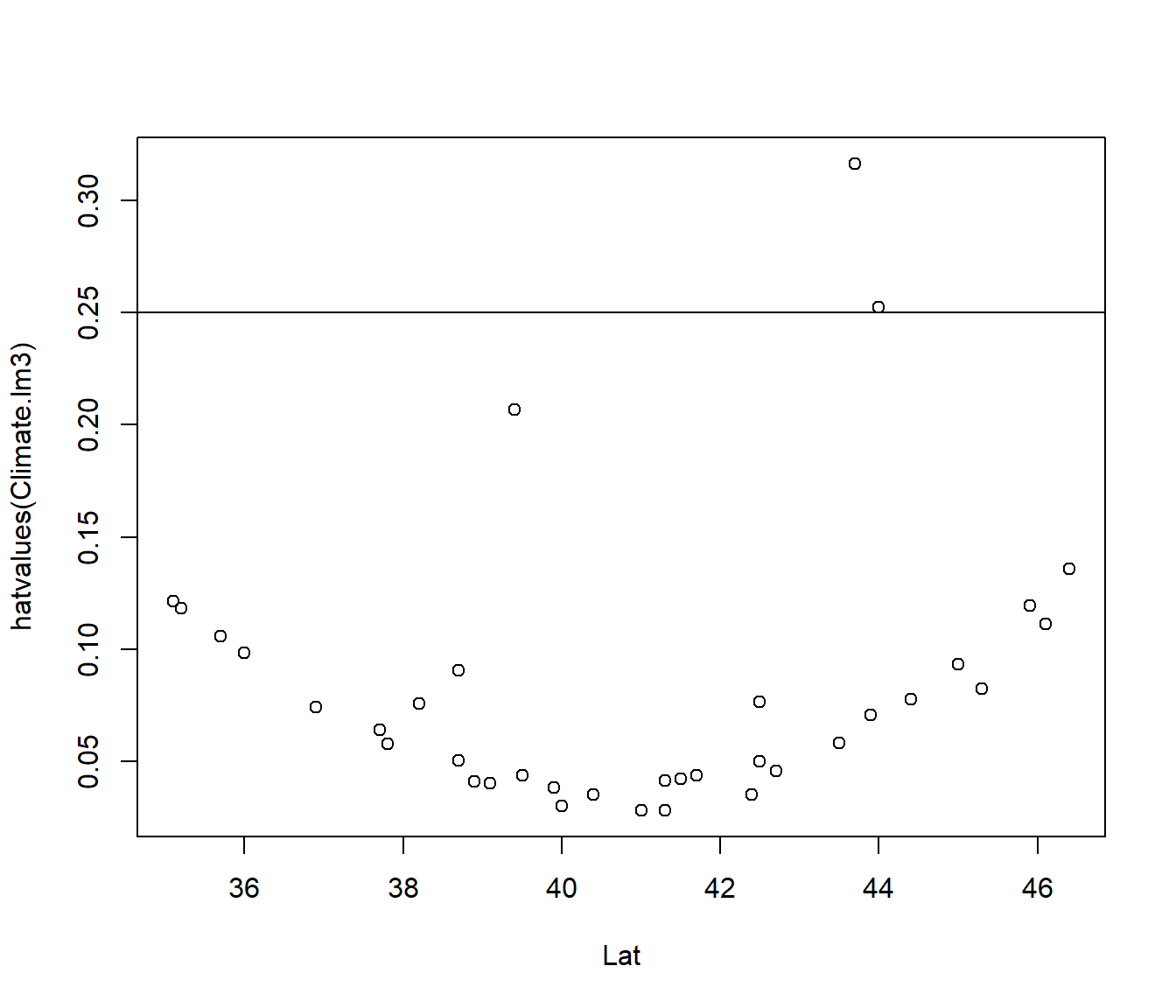
plot(hatvalues(Climate.lm3) ~ Height, data = Climate)
abline(h = 3 * length(coef(Climate.lm3))/nrow(Climate))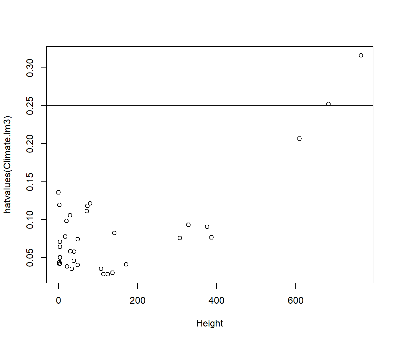
The leverage is related to \((\frac{x-\bar x}{sd(x)})^2\) combined across each predictor in the the model. So the graph has a characteristic quadratic shape for most of the points.
The first graph indicates that high leverage is not related to Lat. The second graph indicates it is explained by extreme values for Height.
Occasionally you get a point which is high leverage although it is not extreme in either variable. In that case it is because the combination of the predictor variables is unusual.
9.10 Interpreting Slopes from a Multiple Regression
Suppose we compare the coefficients from
- the simple linear regression of MnJlyTemp on Lat, to those produced by
- the multiple regression of MnJlyTemp on Lat and Height.
(Intercept)         Lat
34.4212725 -0.6618663 (Intercept) Lat Height
32.878836627 -0.600512089 -0.007198381 We see the slope associated with Lat is a bit different. Why?
The answer is that Lat and Height are slightly correlated
so the presence of Height in the model means Lat does not need to explain MnJlyTemp all by itself. Since there are more very high places in the South Island than in the North Island, some of the trend with Lat is taken away by including Height.
So we settle for the following interpretation:
In a combined regression model \[Y = \beta_0 + \beta_1 x_1 + \beta_2 x_2\]
we interpret \(\beta_1\) the rate of change of y per unit increase of \(x_1\) if \(x_2\) is held constant.
Similarly we interpret \(\beta_2\) the rate of change of y per unit increase of \(x_2\) if \(x_1\) is held constant.
We will see in later lectures that if adding a new variable such as \(x_2\) into a model makes a big difference to the slope estimates, then it may be a good idea to include it, even if its P-value did not quite meet the P<0.05 rule.
9.11 Confidence intervals for coefficients and Prediction intervals
These are calculated the same way for a multiple regression as was done for a simple linear model.
Note that in order to make point or interval estimates, you need to state which values are associated with which variables and put them in a data.frame().
                   2.5 %       97.5 %
(Intercept) 27.928209206 37.829464049
Lat         -0.721909066 -0.479115112
Height      -0.009139715 -0.005257046
x0 <- data.frame(Lat = 40.3525, Height = 20)
# Predicting Mean July Temperature for Palmerston North
predict(Climate.lm3, newdata = x0, interval = "prediction", level = 0.95) fit lwr upr
1 8.502705 6.180698 10.82471