Lecture 27 Variable Selection
27.1 Variable selection
In previous lectures we have looked at tests for single explanatory variables and groups of explanatory variables.
Often, however, a statistician will simply want to know what is the best group of explanatory variables for describing the response.
In this lecture we will consider various criteria for model selection, and cover an example on finding a suitable variable set “by hand”.
27.2 Overfitting and Underfitting
We begin by considering the following question: Should all the explanatory variables be used, or should some be omitted?
Why might we want to omit variables?
Perhaps we want to detect variables which affect the response but avoid collecting unnecessary measurements in the future. This is called variable screening
Perhaps we want to predict from the model. Our predictions will be less accurate if the model is incorrectly specified.
We first consider the risks and benefits of including a predictor that might have coefficient \(\beta=0\).
27.3 Dropping or Including Variables that have \(\beta=0\)
Suppose we have a regression model with several variables. We might suspect one has regression coefficient \(\beta=0\). Should we drop it?
Some mathematical theory shows that if we omit a variable which (truly) has regression coefficient \(\beta=0\) then
Variances of the remaining regression coefficients are reduced
Variances of predictions from the model at any point \(x_0\) are reduced.
Both these things are good.
Conversely if we include a variable whose coefficient \(\beta=0\) this increases these variances unnecessarily. This is called overfitting. We want to avoid this.
27.4 Dropping or Including Variables that have \(\beta \ne 0\)
On the other hand suppose we make a mistake and omit a variable that has regression coefficient \(\ne 0\).
Then we have the opposite problem, called underfitting. Mathematical theory shows the consequence of underfitting is that
if the wrongly-omitted variables are correlated with the remaining variables then the expected values of the remaining regression coefficients \(\beta_0,\beta_1,...\beta_{p-1}\) are biased. (i.e. may be a too big or too small).
Whether or not the omitted variables are correlated with the existing ones, the predictions \(\hat y_i\) are biased.
Both these things are bad!
In practice we do not know if parameters are zero. We could use a hypothesis test to help us decide, but this is not a definitive answer.
27.5 A Numerical Illustration of Under and Overfitting
In this artificial example, we consider an industrial process whose Yield is thought to depend on the process temperature at stage A of the process, and possibly also on the temperature at stage B.
i.e. We consider the model \[ Y=\beta_0 + \beta_1 A+ \beta_2 B +\varepsilon.\]
We will assume the values of \(A\) and \(B\) and \(\varepsilon\) are given in the data below. The errors are random \(\varepsilon \sim \mbox{Normal}(0, 1)\).
What we want to know is, what are the implications of using an incorrect model, i.e. incorrect assumptions about the \(\beta\)s. To understand the implications, we simulate two scenarios.
27.6 Scenario 1: \(\beta_0=50\), \(\beta_1=10\) and \(\beta_2=0\).
For this illustration, the correct model doesn’t depend on \(B\) at all: \[Y = 50 + 10 A + \varepsilon\]
The following shows the result of modelling \(Y\) by (1) \(A\) alone and (2) by \(A\) and \(B\).
dat <- sim |>
    mutate(Y = 50 + 10 * A + epsilon)
lm1 = lm(Y ~ A, data = dat)
lm2 = lm(Y ~ A + B, data = dat)
lst(lm1, lm2) |>
    map_dfr(tidy, .id = "model")
# A tibble: 5 × 6
model term estimate std.error statistic p.value
<chr> <chr> <dbl> <dbl> <dbl> <dbl>
1 lm1 (Intercept) 49.3 2.03 24.2 3.43e-15
2 lm1 A 10.0 0.112 89.4 2.71e-25
3 lm2 (Intercept) 48.8 2.14 22.8 3.43e-14
4 lm2 A 9.76 0.338 28.9 7.01e-16
5 lm2 B 0.290 0.350 0.827 4.19e- 1Adding the unnecessary variable doesn’t introduce bias (\(\hat\beta_1 \approx 10\)), but the standard error of \(\hat\beta_1\) is higher in the misspecified model.
27.7 Scenario 2: \(\beta_0=50\), \(\beta_1=5\) and \(\beta_2=5\).
We consider the model where \(Y\) depends on both \(A\) and \(B\), \[ Y = 50 + 5 A + 5 B + \varepsilon \]
dat <- sim |>
    mutate(Y = 50 + 5 * A + 5 * B + epsilon)
lm1 = lm(Y ~ A, data = dat)
lm2 = lm(Y ~ A + B, data = dat)
lst(lm1, lm2) |>
    map_dfr(tidy, .id = "model")
# A tibble: 5 × 6
model term estimate std.error statistic p.value
<chr> <chr> <dbl> <dbl> <dbl> <dbl>
1 lm1 (Intercept) 57.8 7.57 7.63 4.74e- 7
2 lm1 A 9.58 0.418 22.9 8.94e-15
3 lm2 (Intercept) 48.8 2.14 22.8 3.43e-14
4 lm2 A 4.76 0.338 14.1 8.48e-11
5 lm2 B 5.29 0.350 15.1 2.75e-11In the first model, \(B\) is wrongly ignored and \(A\) is both biased and has a larger standard error. In the second model, the values of \(\hat\beta_1\) and \(\hat\beta_2\) are close to the true ones and the standard errors are the same as in the second analysis of Scenario 1.
27.8
In summary, if we omit a needed variable then we may introduce bias into our estimation.
The big problem with bias is that there may be no sign that we have a mistake.
In some cases we don’t even have the needed variable, so we can’t try it in the model.
At least in case 1, when we wrongly enter an unnecessary variable, it doesn’t bias our estimates, just increases our standard errors. So at least we know exactly how bad things are. But with an omitted variable we don’t know how bad things are.
For this reason, we may decide to err on the side of caution and add in variables even if we are uncertain about their relevance. Then at least we can avoid bias.
27.9 Model Selection: Bias and Variance
Model selection, then, comes down to balancing the effects of variance and bias.
If we omit a variable, it may dramatically decrease the variance of the other parameter estimates. This is a plus.
But if the variable is important, then the other parameter estimates may be biased. This is a minus.
So what should we choose? There is no settled rule for every circumstance, but in general we should probably be more concerned to avoid bias (especially since we don’t know how bad this is!) than to avoid a small increase in variance (at least we do know how bad it is - we can see the standard errors.)
Consequently we may decide to err on the side of including variables with P-values a little bigger than 0.05, especially if they seem to induce a sizeable change in the other coefficient estimates. This is another thing to watch out for in model selection.
27.10 Review of Model Selection Criteria
There are a number of measures we can use for model selection:
Coefficient of determination \(R^2\)
Adjusted Coefficient of determination \(R^2_{Adj}\)
Residual Standard Error \(S\)
\(P\)-values of individual coefficients
Each of these are slightly different, so it pays to consider more than one.
27.11 Coefficient of determination \(R^2\)
Recall that this is the proportion of total variation which is explained by the model. (Alternatively, 1 minus the ratio of unexplained variation to total variation): \[ R^2 = \frac{SS_{Regn}}{SST} = 1 - \frac{\sum(y_i-\hat y_i)^2}{\sum(y_i-\bar y)^2}. \] \(R^2\) is useful for comparing two models with the same number of regression parameters. If models have different numbers of regression parameters we use the adjusted version.
27.12 Adjusted Coefficient of determination \(R^2_{Adj}\)
Recall that this is 1 minus the ratio of Mean Square Error to Mean Square Total: \[ R^2_{Adj} = 1 - \frac{MSE}{MST} = 1 - \frac{\sum(y_i-\hat y_i)^2/(n-p)}{\sum(y_i-\bar y)^2/(n-1)}.\] When considering adding a variable to a regression, the \(R^2_{Adj}\) goes up if the variable is “worth” at least one row of data (one degree of freedom), which is a pretty low bar to cross.
But at least if a variable can’t meet that rule then we know to exclude it.
27.13 Residual Standard Error \(S\)
This is the standard deviation of the residuals, \[ S = \frac{1}{n-p}\sum{(y_i - \hat y_i)^2} \] or in other words the standard deviation of how the \(y_i\)s vary around the model predictions. We might choose to include a variable if it reduces the \(S\).
27.14 \(P\)-value for individual coefficients
We usually prefer models that only include variables with coefficient \(P\)-value is small (e.g. \(< 0.05\)).
However the “0.05” criterion is somewhat arbitrary and occasionally we allow in variables with slightly higher \(P\)-values to potentially reduce bias.
27.15 Example: Model Selection for Climate Data
We wish to model the mean temperature in July (winter) in Aotearoa New Zealand using data from 36 towns. We have information on location (latitude, longitude, height (elevation), whether they’re by the sea or in the North island) as well as climate information (mean temperature in January, total sunshine hours and total rainfall).
# A tibble: 36 × 10
   Place      Lat  Long MnJanTemp MnJlyTemp  Rain   Sun Height   Sea NorthIsland
   <chr>    <dbl> <dbl>     <dbl>     <dbl> <dbl> <dbl>  <dbl> <dbl>       <dbl>
 1 Kaitaia   35.1  173.      19.3      11.7  1418  2113     80     1           1
 2 Kerikeri  35.2  174       18.9      10.8  1682  2004     73     1           1
 3 Dargavi…  36    174.      18.6      10.7  1248  1956     20     1           1
 4 Whangar…  35.7  174.      19.7      11    1600  1925     29     1           1
 5 Auckland  36.9  175.      19.4      11    1185  2102     49     1           1
 6 Tauranga  37.7  176.      18.5       9.3  1349  2277      4     1           1
 7 Hamilton  37.8  175.      17.8       8.3  1201  2006     40     0           1
 8 Rotorua   38.2  176.      17.5       7.3  1439  1948    307     0           1
 9 Gisborne  38.7  178       18.7      13.6  1058  2204      4     1           1
10 Taupo     38.7  177.      17.3       6.5  1178  2021    376     0           1
# ℹ 26 more rows
27.16 Climate Exploratory Data Analysis
climate |>
    pivot_longer(-c(Place, MnJlyTemp)) |>
    ggplot() + geom_point(mapping = aes(x = value, y = MnJlyTemp)) + facet_wrap(vars(name),
    scales = "free_x", ncol = 4)
27.17 Higher winter temperature associations
- Lower elevations (height)
- Lower latitudes (further north)
- Higher longitudes (further east - recall how Ao/NZ is oriented on a map - possibly correlation with latitude, will check next!)
- Higher summer temperatures
- North island (could just be latitude?)
- Increased rainfall - up to a point! (subtropical vs rainy westcoast - interaction with Island/latitude??)
- Closeness to the sea
- Increased sunshine hours
Many of these are likely correlated.
27.18 Climate: Latitude/Longitude and North vs South
ggplot(climate) + geom_point(mapping = aes(x = Long, y = -Lat, shape = as_factor(NorthIsland),
    col = MnJlyTemp)) + geom_text(mapping = aes(x = Long, y = -Lat, label = Place),
    size = 2, hjust = "right", nudge_x = 0.1, nudge_y = 0.2) + coord_equal()
27.19 📊 Climate: Latitude/Longitude and North vs South
Ok, so we can see that the temperature is being driven by latitude (further north is warmer) - the longitude effect is possibly just due to orientation. It’s clear there’s an elevation (height) effect as well, though that is possibly confounded with whether the town is close to the sea (it can’t really be both!)
So we’d expect some collinearity here and figuring out which are the best variables to be used might take a bit of playing!
We’ll start with Latitude, then add in Height and Sea:
27.20 Climate: model 1 output
Call:
lm(formula = MnJlyTemp ~ Lat, data = climate)

Residuals:
    Min      1Q  Median      3Q     Max
-3.6992 -0.9786  0.1566  1.0588  4.7930

Coefficients:
            Estimate Std. Error t value Pr(>|t|)
(Intercept) 34.42127    3.94299   8.730 3.35e-10 ***
Lat         -0.66187    0.09613  -6.885 6.25e-08 ***
---
Signif. codes:  0 '***' 0.001 '**' 0.01 '*' 0.05 '.' 0.1 ' ' 1

Residual standard error: 1.822 on 34 degrees of freedom
Multiple R-squared:  0.5824,    Adjusted R-squared:  0.5701
F-statistic: 47.41 on 1 and 34 DF,  p-value: 6.25e-08
27.21 Climate: model 2 output
Call:
lm(formula = MnJlyTemp ~ Lat + Height, data = climate)

Residuals:
    Min      1Q  Median      3Q     Max
-2.0607 -0.6215 -0.1021  0.5145  3.9898

Coefficients:
              Estimate Std. Error t value Pr(>|t|)
(Intercept) 32.8788366  2.4333203  13.512 5.30e-15 ***
Lat         -0.6005121  0.0596687 -10.064 1.38e-11 ***
Height      -0.0071984  0.0009542  -7.544 1.12e-08 ***
---
Signif. codes:  0 '***' 0.001 '**' 0.01 '*' 0.05 '.' 0.1 ' ' 1

Residual standard error: 1.121 on 33 degrees of freedom
Multiple R-squared:  0.8467,    Adjusted R-squared:  0.8374
F-statistic: 91.14 on 2 and 33 DF,  p-value: 3.639e-14
27.22 Climate: model 3 output
Call:
lm(formula = MnJlyTemp ~ Lat + Height + Sea, data = climate)

Residuals:
    Min      1Q  Median      3Q     Max
-1.7969 -0.4792 -0.0299  0.5042  3.7850

Coefficients:
             Estimate Std. Error t value Pr(>|t|)
(Intercept) 31.290016   2.290747  13.659 6.71e-15 ***
Lat         -0.587826   0.054584 -10.769 3.59e-12 ***
Height      -0.005121   0.001147  -4.463 9.38e-05 ***
Sea          1.294326   0.466063   2.777  0.00909 **
---
Signif. codes:  0 '***' 0.001 '**' 0.01 '*' 0.05 '.' 0.1 ' ' 1

Residual standard error: 1.022 on 32 degrees of freedom
Multiple R-squared:  0.8765,    Adjusted R-squared:  0.8649
F-statistic: 75.69 on 3 and 32 DF,  p-value: 1.275e-14
27.23 Climate: First three predictors.
For these first three predictors:
- They have significant p-values
- \(S\) has gone down each time
- The adjusted \(R^2\) and has gone up each time.
There is no reason to doubt that Lat, Height and Sea should all be included.
Also note the regression coefficient for Height altered by about 2 standard errors, which suggests that Sea is correcting for bias, all the more reason for including it.
This makes sense - sea level towns will mostly have a very low height, but there’ll also be an additional warming effect of being close to the sea.
27.24 Climate: Adding island
Call:
lm(formula = MnJlyTemp ~ Lat + Height + Sea + NorthIsland, data = climate)

Residuals:
    Min      1Q  Median      3Q     Max
-1.2667 -0.5054 -0.2098  0.4707  3.4088

Coefficients:
             Estimate Std. Error t value Pr(>|t|)
(Intercept) 21.378217   4.637932   4.609 6.56e-05 ***
Lat         -0.375517   0.101816  -3.688 0.000862 ***
Height      -0.004416   0.001109  -3.981 0.000385 ***
Sea          1.803422   0.483327   3.731 0.000766 ***
NorthIsland  1.559710   0.647795   2.408 0.022193 *
---
Signif. codes:  0 '***' 0.001 '**' 0.01 '*' 0.05 '.' 0.1 ' ' 1

Residual standard error: 0.9526 on 31 degrees of freedom
Multiple R-squared:  0.8959,    Adjusted R-squared:  0.8825
F-statistic: 66.73 on 4 and 31 DF,  p-value: 8.723e-15
Same conclusions as before, we should include NorthIsland
Including it has induced big changes in the coefficients (especially Lat) which again is evidence it is important.
Why do you think adding North vs South island is useful over and above Latitude? Wouldn’t Latitude do everything here??
27.25 Climate: Adding Rain
Call:
lm(formula = MnJlyTemp ~ Lat + Height + Sea + NorthIsland + Rain,
    data = climate)

Residuals:
    Min      1Q  Median      3Q     Max
-1.2829 -0.5042 -0.1944  0.4422  3.4651

Coefficients:
              Estimate Std. Error t value Pr(>|t|)
(Intercept) 19.6651523  4.6317227   4.246 0.000194 ***
Lat         -0.3437001  0.1009517  -3.405 0.001900 **
Height      -0.0049792  0.0011322  -4.398 0.000127 ***
Sea          1.6435808  0.4802716   3.422 0.001814 **
NorthIsland  1.7682036  0.6430084   2.750 0.010003 *
Rain         0.0003583  0.0002170   1.651 0.109182
---
Signif. codes:  0 '***' 0.001 '**' 0.01 '*' 0.05 '.' 0.1 ' ' 1

Residual standard error: 0.9271 on 30 degrees of freedom
Multiple R-squared:  0.9046,    Adjusted R-squared:  0.8887
F-statistic:  56.9 on 5 and 30 DF,  p-value: 2.11e-14
The Rain variable is not significant (P=0.1) which goes against including Rain. However \(S\) has gone down and the adjusted R-squared has gone up. So we may decide that if our aim is to predict for new data, then we should include this variable in the model.
27.26 Climate: Adding Longitude
lm6 = lm(MnJlyTemp ~ Lat + Height + Sea + NorthIsland + Rain + Long, data = climate)
lm6 |>
    summary()
Call:
lm(formula = MnJlyTemp ~ Lat + Height + Sea + NorthIsland + Rain +
    Long, data = climate)

Residuals:
    Min      1Q  Median      3Q     Max
-1.3360 -0.4832 -0.1712  0.4008  3.2814

Coefficients:
              Estimate Std. Error t value Pr(>|t|)
(Intercept)  6.8938252 21.1286658   0.326 0.746557
Lat         -0.3272942  0.1053819  -3.106 0.004216 **
Height      -0.0050077  0.0011449  -4.374 0.000144 ***
Sea          1.6381187  0.4853578   3.375 0.002113 **
NorthIsland  1.5548897  0.7352242   2.115 0.043156 *
Rain         0.0004002  0.0002295   1.744 0.091750 .
Long         0.0701947  0.1132443   0.620 0.540196
---
Signif. codes:  0 '***' 0.001 '**' 0.01 '*' 0.05 '.' 0.1 ' ' 1

Residual standard error: 0.9368 on 29 degrees of freedom
Multiple R-squared:  0.9059,    Adjusted R-squared:  0.8864
F-statistic: 46.51 on 6 and 29 DF,  p-value: 1.402e-13
At this point all the indications are bad: The P-value for Long is >0.5, the adjusted R-squared has gone down and S has gone up.
So we should not include Long in the model.
27.27 📊 Climate Data Case Study — Key Takeaways
Goal: Predict NZ July temperature from location and climate covariates
Final model path: MnJlyTemp ~ Lat + Height + Sea + NorthIsland + Rain
Model progression
| Model | Variables | \(R^2_{\text{Adj}}\) | \(S\) | Key variable \(p\) |
|---|---|---|---|---|
| 1 | Lat | 0.570 | 1.82 | < 0.001 |
| 2 | + Height | 0.837 | 1.12 | < 0.001 |
| 3 | + Sea | 0.865 | 1.02 | < 0.001 |
| 4 | + NorthIsland | 0.883 | 0.95 | < 0.001 |
| 5 | + Rain | 0.889 | 0.92 | 0.10 |
| 6 | + Long | 0.886 | 0.93 | 0.54 |
27.28 📊 Climate Data Case Study — Key Takeaways Continued
🔍 What to watch for
- Coefficient shifts after adding variables indicate possible bias correction
- Look for agreement among criteria, not just \(p\) values
- Longitude rejected: \(p>0.5\), \(R^2_{\text{Adj}}\downarrow\), \(S\uparrow\)
🚨 Warning signs
- Large coefficient changes when adding or removing variables → potential bias
- Sole reliance on \(p<0.05\) can miss important predictors
- Ignoring \(R^2_{\text{Adj}}\) and \(S\) gives an incomplete picture
- Criteria in conflict → justify with domain knowledge and prediction error
Recommendation:
Retain Lat, Height, Sea, NorthIsland. Retain Rain when prediction accuracy is the goal, as it is here.
27.29 🤔 Done? 🤔
Not so fast! We now have a model, but is it any good? Does it meet our LINE assumptions?
After variable selection, you must check if the final model satisfies the assumptions of linear regression. Let’s check the diagnostics for our chosen model:
lm(MnJlyTemp ~ Lat + Height + Sea + NorthIsland + Rain, data = climate).
27.30 Final Model Diagnostics
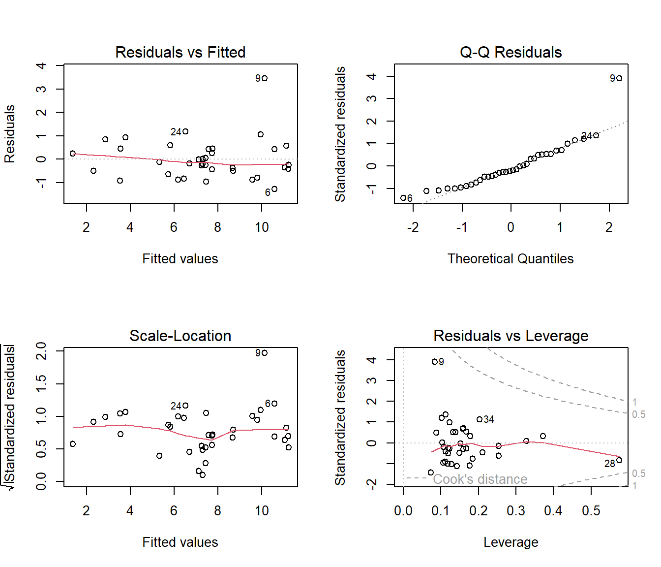
27.30.1 Interpretation of Diagnostic Plots:
- Residuals vs. Fitted: The red line is nearly flat and the points are randomly scattered around 0. This looks good and suggests the linearity assumption holds. No obvious patterns.
- Normal Q-Q: The points fall very closely along the dashed line except one point (9). This indicates the residuals are normally distributed, which is great.
- Scale-Location: The points are randomly scattered and the red line is relatively flat. This confirms the assumption of equal variance (homoscedasticity).
- Residuals vs. Leverage: No points appear outside of the dashed Cook’s distance lines, meaning we don’t have any single data points that are overly influential on our results.
Conclusion: Our final model not only makes intuitive sense but also passes the standard diagnostic checks! It appears to be a robust and reliable model.