Lecture 25 The General Linear Model
We have mostly focused on (i) models containing just numerical covariates (linear regression models) and (ii) models containing just factors (‘ANOVA type’ models).
Naturally there will be situations in which we wish to model a response in terms of both numerical covariates and factors. We saw this in the case of the English Exam data.
Generalizing factorial and regression models to include models with potentially both factors and numerical covariates produces the class of models (historically) referred to as General Linear Models.
The abbreviation GLM was used for these models for many years, and still is in some software. R uses this acronym to refer to generalised linear models which are covered in another course. As a consequence, we often find some confusion, but all linear models fit into the wider group of generalised linear models
We will look at general linear models in this lecture.
25.1 General Linear Models as Regressions
As we saw when we looked at factorial models, any factor can be coded using dummy variables so as to produce a linear regression model.
It follows that any general linear model can be fitted as a linear regression.
All the ideas about least squares estimation, fitted values and residuals remain unchanged.
25.2 Models with a Single Factor and Covariate
In order to understand how to use and interpret models with a combination of factors and numerical covariates, consider the simple case where we have a response variable, y, a covariate x and a factor A.
There are a number of different models that we could fit.
- differently sloped regressions for each level of A,
- parallel regressions at different levels of A,
- single regression model,
- model with zero slope, but distinct intercept for each Level of A, and
- a null model having zero slope and common intercept.

25.3 Separate Regressions at Different Levels of A
\[Y_{ij} = \mu + \alpha_i + \beta_i x_{ij} + \varepsilon_{ij}\]
Note: intercept and slope depends on factor level i.
Treatment constraint fixes \(\alpha_1 = 0\).
R formula is Y ~ A + A:x
Here the notation of an interaction between the covariate and the factor is telling R to allow the regression slope to depend on the factor level.
25.4 Parallel Regressions at Different Levels of A
\[Y_{ij} = \mu + \alpha_i + \beta x_{ij} + \varepsilon_{ij}\]
Note: constant slope, but intercept depends on factor level i.
Treatment constraint sets \(\alpha_1 = 0\).
R formula is Y ~ A + x
25.5 Single Regression Model
\[Y_{ij} = \mu + \beta x_{ij} + \varepsilon_{ij}\]
Note: factor A plays no role here.
R formula is the familiar Y ~ x
Technical aside:
Another possible model would be different regression slopes but a common intercept, but this is not commonly used.
25.6 Interpretation of Linear Model Formulae
The ideas just presented can be extended in a natural fashion to models with two or more factors and covariates.
Suppose that the R formula is Y ~ A + A:B + A:x + z, where A and B are factors, and x and z are covariates. Then the model is defined by:
\[Y_{ijk} = \mu +\alpha_i + \beta_{ij} + \gamma_i x_{ijk} + \delta z_{ijk} + \varepsilon_{ijk}.\]
Suppose that the R formula is Y ~ A*B + A:x
This model is defined by \(Y_{ijk} = \mu +\alpha_i + \beta_j + (\alpha\beta)_{ij} + \gamma_i x_{ijk} + \varepsilon_{ijk}.\)
Suppose that the R formula is Y ~ A + A:x + B + B:z
This model is defined by \(Y_{ijk} = \mu +\alpha_i + \beta_j + \gamma_{i} x_{ijk} + \delta_j z_{ijk} + \varepsilon_{ijk}.\)
25.7 Samara
Samara are small winged fruit on maple trees.
In Autumn these fruit fall to the ground, spinning as they go.
Research on the aerodynamics of the fruit has applications for helicopter design.

25.8 Linear Models for Samara Data
In one study the following variables were measured on individual samara:
Velocity: speed of fallTree: data collected from 3 treesLoad: ‘disk loading’ (an aerodynamical quantity based on each fruit’s size and weight).
The aim of this Case Study is to model Velocity in terms of Load (a numerical covariate) and Tree (a factor).
25.9 Samara Data: R Code
'data.frame':   35 obs. of  3 variables:
 $ Tree    : int  1 1 1 1 1 1 1 1 1 1 ...
 $ Load    : num  0.239 0.208 0.223 0.224 0.246 0.213 0.198 0.219 0.241 0.21 ...
$ Velocity: num 1.34 1.06 1.14 1.13 1.35 1.23 1.23 1.15 1.25 1.24 ...N.B. It might prove useful to have the values of Tree as both a numeric and a factor variable.
25.10 Samara Data: Plot of Data
Samara |>
    ggplot(mapping = aes(y = Velocity, x = Load)) + geom_point(mapping = aes(col = TreeF,
    pch = TreeF))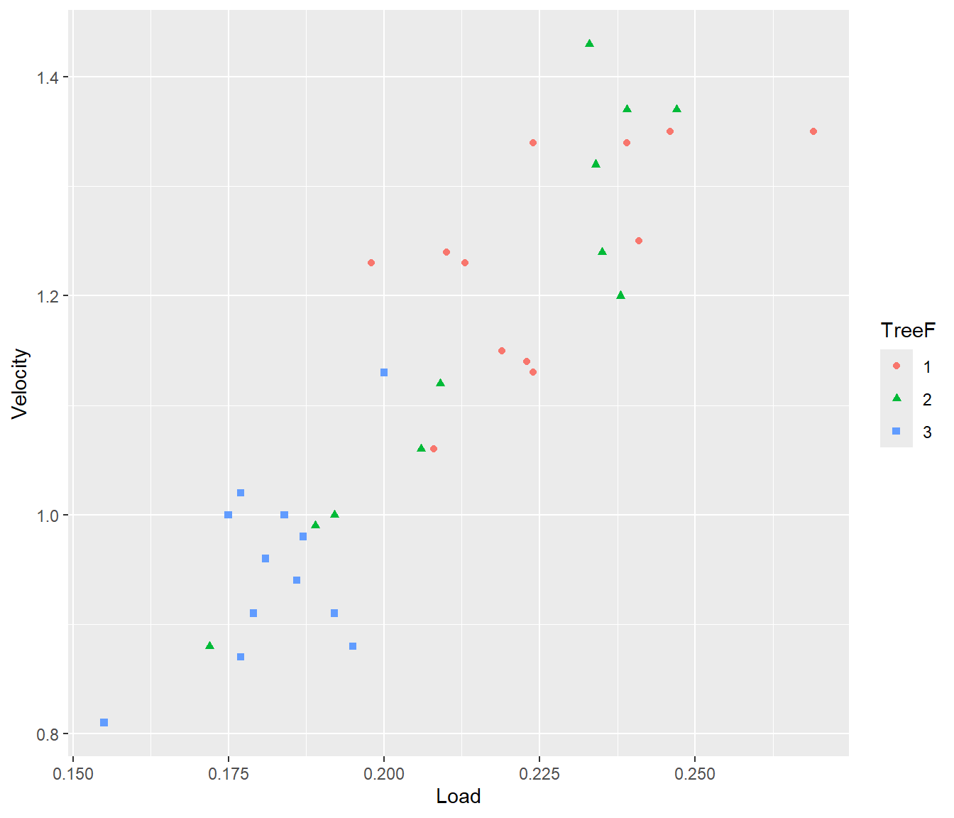
Figure 25.1: Scatter plot of data with different colours and plotting symbols used to distinguish data from different trees.
25.11 Model Fitting
We will fit a model with separate regression lines at different levels of TreeF.
The following shows the effect parameterising the model two ways:
The first way gives estimates for the intercept and slope for each line separately. We do this by excluding the Load term from the model formula, and including only the interaction between TreeF and Load.
Call:
lm(formula = Velocity ~ TreeF + TreeF:Load, data = Samara)

Residuals:
      Min        1Q    Median        3Q       Max
-0.120023 -0.049465 -0.001298  0.049938  0.145571

Coefficients:
            Estimate Std. Error t value Pr(>|t|)
(Intercept)   0.5414     0.2632   2.057   0.0488 *
TreeF2       -0.8408     0.3356  -2.505   0.0181 *
TreeF3       -0.2987     0.4454  -0.671   0.5078
TreeF1:Load   3.0629     1.1599   2.641   0.0132 *
TreeF2:Load   6.7971     0.9511   7.147 7.26e-08 ***
TreeF3:Load   3.8834     1.9672   1.974   0.0580 .
---
Signif. codes:  0 '***' 0.001 '**' 0.01 '*' 0.05 '.' 0.1 ' ' 1

Residual standard error: 0.07554 on 29 degrees of freedom
Multiple R-squared:  0.8436,    Adjusted R-squared:  0.8167
F-statistic: 31.29 on 5 and 29 DF,  p-value: 7.656e-11
Note the first model has TreeF1:Load, and the coefficients for TreeF2:Load and TreeF3. Load are tested against the hypotheses that the slope is zero for each of those trees. This may not be a sensible hypothesis.
25.12
The second way specifies a baseline (for TreeF1), and then adjustments to the intercept and slope for the second and third line. The second way gives us insight into where there are significant differences to the baseline, (if any).
Call:
lm(formula = Velocity ~ TreeF * Load, data = Samara)

Residuals:
      Min        1Q    Median        3Q       Max
-0.120023 -0.049465 -0.001298  0.049938  0.145571

Coefficients:
            Estimate Std. Error t value Pr(>|t|)
(Intercept)   0.5414     0.2632   2.057   0.0488 *
TreeF2       -0.8408     0.3356  -2.505   0.0181 *
TreeF3       -0.2987     0.4454  -0.671   0.5078
Load          3.0629     1.1599   2.641   0.0132 *
TreeF2:Load   3.7343     1.5000   2.490   0.0188 *
TreeF3:Load   0.8205     2.2837   0.359   0.7220
---
Signif. codes:  0 '***' 0.001 '**' 0.01 '*' 0.05 '.' 0.1 ' ' 1

Residual standard error: 0.07554 on 29 degrees of freedom
Multiple R-squared:  0.8436,    Adjusted R-squared:  0.8167
F-statistic: 31.29 on 5 and 29 DF,  p-value: 7.656e-11
As usual, the treatment constraint is used by default for TreeF (the factor version of Tree). Hence the Intercept listed under the coefficients is the intercept for TreeF1, with adjustments for treeF2 and 3 given in the summary table. The relevant hypothesis tests are for whether the intercepts and slopes are the same or different to that of the baseline.
25.13 Conclusions
Either way we get the fitted model is as follows:
\[\begin{aligned} &\mbox{Tree 1}&~~~E[ \mbox{Velocity}] = 0.541 + 3.06 \mbox{Load}\\ &\mbox{Tree 2}&~~~E[ \mbox{Velocity}] = -0.299 + 6.80 \mbox{Load}\\ &\mbox{Tree 3}&~~~E[ \mbox{Velocity}] = 0.242 + 3.88 \mbox{Load}\end{aligned}\]
Check that you can get the same numbers with either parameterisation.
25.13.1 Checking models
Two different parameterisations of the same model will have different coefficients in the summary() output.
They will have to have the same number of coefficients though.
If you need to convince yourself that two different parameterisations lead to the same underlying model, look at the fitted values for each parameterisation.
Same fitted values means same residuals etc.