Lecture 39 Serial Correlation
Loading required package: zoo
Attaching package: 'zoo'The following objects are masked from 'package:base':
as.Date, as.Date.numeric39.0.1 Introduction: Autocorrelation
The standard assumption in regression models is that errors are uncorrelated. This means that, once you take out the overall linear trend in the data, then the residuals are randomly scattered. For example, having a high positive residual on one row of the data gives you no clue about whether the residual is likely to be positive or negative on the next row.
If this assumption is untrue then we describe the data as having “correlated errors”. When it occurs because observations have a natural sequential order, this correlation is referred to as serial correlation, or autocorrelation.
Autocorrelation (usually) implies that adjacent residuals will tend to be similar.
This may be because of some omitted variable. For example spatial (“space–ial”) autocorrelation may occur in agriculture because adjacent plots of ground have similar soil, drainage and weather patterns, compare to plots in different areas. Or district-by-district medical data may show autocorrelation in cases of disease, again because of weather or because of similarity of ethnic background and lifestyle of people in adjacent districts.
Temporal autocorrelation (i.e. in time) in stock or exchange rate prices may also be because of omitted variables. For example, prices may be relatively high one week because of certain economic conditions etc. Then unless those conditions have suddenly changed the prices are likely to remain relatively high the following week.
The point is that if we were to include information about the omitted variable in the analysis, then the apparent autocorrelation would disappear.
However autocorrelation may also occur because of some genuine infectious-type behaviour. For example:
in agriculture, if a field of barley is diseased, then the adjacent field may be infected by the first one;
in business, if one business fails it may damage the ability of other businesses to keep trading;
in education, if one student uses drugs then other students may be encouraged to try them, etc.
Whilst adding an appropriate variable to the model may remove the apparent autocorrelation in some situations, there is less we can do about infectious behaviour. We have to live with it and adjust our analysis.
If the errors are correlated then this is both a nuisance (makes the analysis harder) and an opportunity (maybe there is information in the data we can exploit).
39.1 Positive or Negative Autocorrelation?
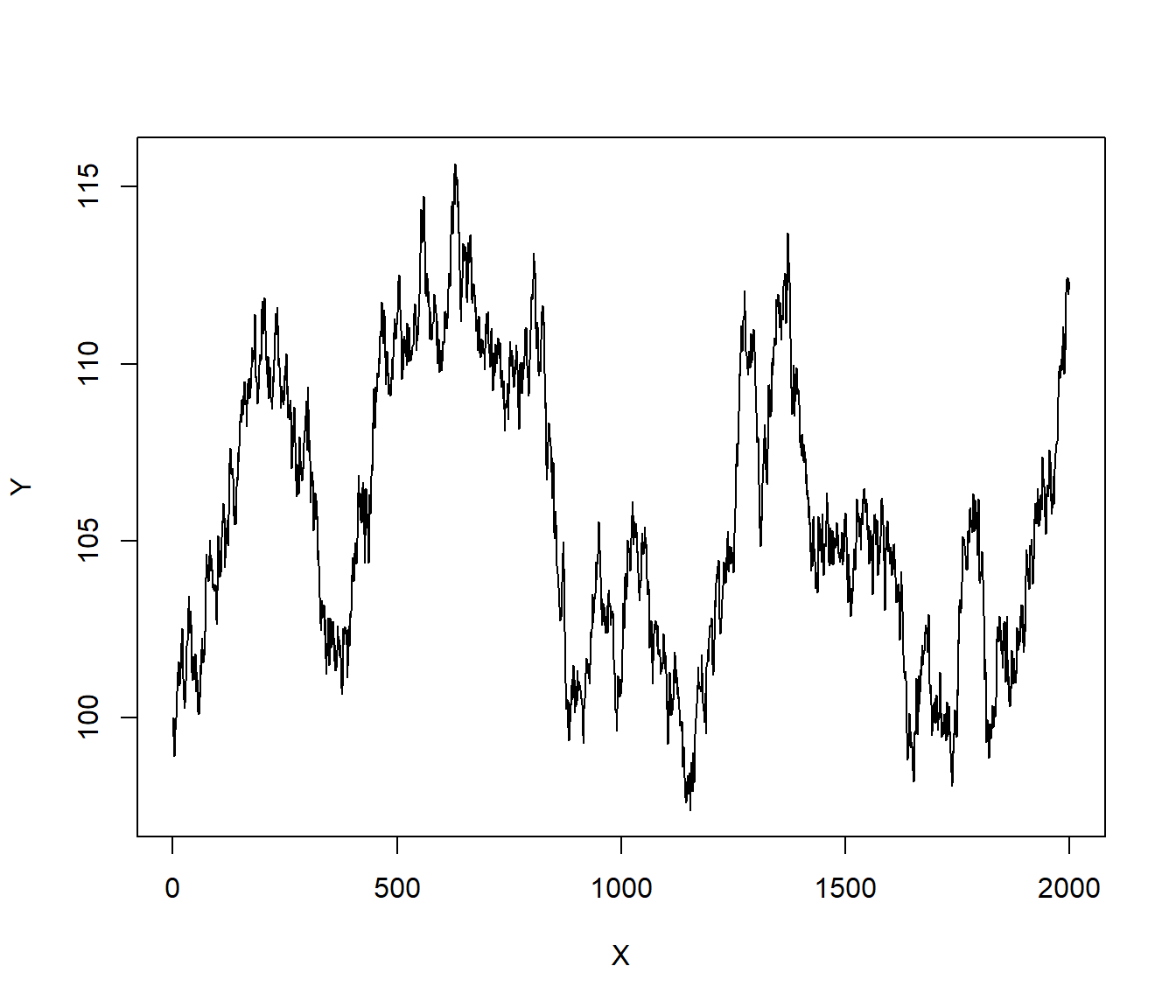
• When data are positively autocorrelated, high positive residuals tend to be followed by more positive residuals, and high negative residuals tend to be followed by further negative ones.
The result is that the residuals show a long slow wandering behaviour.
X = 1:2000
err = rnorm(2000, 0, 0.5)
Y = rep(100, 2000)
for (i in 2:2000) Y[i] = Y[i - 1] + err[i]
plot(X, Y, type = "l")
Example. Suppose the stock market is fairly stable and the price of a particular stock is not going anywhere. However by chance someone comes into a lot of cash, and decides to invest in that stock. (Or, alternatively, somebody decides to sell their shares for some reason totally unrelated to the stock). In terms of modelling the stock market, both of these would be regarded as random events. However, if the sale is big enough, others may take notice. In the case of a big purchase, they may think there is some good news in the wings, for the company, and so may decide to buy as well. Then the positive blip in prices is reinforced. (In the alternative case of the big sale, others may think there is something wrong with the company, and so decide to sell their shares as well. Then the negative blip is repeated by more negative blips.)
Both these situations are referred to as positive autocorrelation: the tendency for random blips to be reinforced by blips in the same direction. Eventually, in either case, it will become clear there was no problem with the stock, and the price will return to about normal - the effect will die out.
You can also get negative autocorrelation. This is where figures oscillate above average (or above the trend), below average, above , below, above, …
For example (purely hypothetical?!) Suppose by chance there are far more car accident fatalities than usual one month. This would generally lead to a police blitz on speed/drink driving etc.
As there is more law-enforcement, the public may take more care. This will probably lead to fewer fatalities next month (below average).
However, once the numbers are down, the police will divert resources to some other area of crime. I.e. there will be a relaxation of the blitz.
It is possible that the public will then go back to their old ways. In a really bad situation you would get an oscillatory effect, above and below the long-term mean.
The above example may be a little far-fetched, but we may see oscillatory behaviour in the case of sales of some goods where there is a continual (periodic) demand. (E.g. I started buying my favourite breakfast cereal when it was “on special” and thereafter I buy it every two weeks).
39.2 The Effects of Autocorrelation
Least squares estimates are unbiased but are not efficient.
Basically what this means is that we still expect errors above and below the line to cancel out, but they will take longer to do so (require more data). We can get better estimates using a more sophisticated method than Least Squares, that takes account of the autocorrelation. These better estimates will usually have more reliable standard errors than the Least Squares ones.The estimate of \(\sigma\) and related standard errors that we get from Least Squares may be understated, i.e. the estimated regression parameters would appear to be more accurate than they really are. This is a serious drawback, because we have a problem with accuracy and yet may not realise it.
Confidence intervals and hypothesis tests are not valid (have wrong significance level etc). This is a consequence of the previous point.
In summary, if we have autocorrelation then we need to take action. What action we take depends on whether the autocorrelation is apparent (due to omitted variables) or “pure autocorrelation”. The former is something we can start to deal with in this course. The latter may require a transformation of the data, or the application of specialist Time Series techniques. Next we consider a numerical example.
39.3 Example: Consumer Expenditure and Money Stock
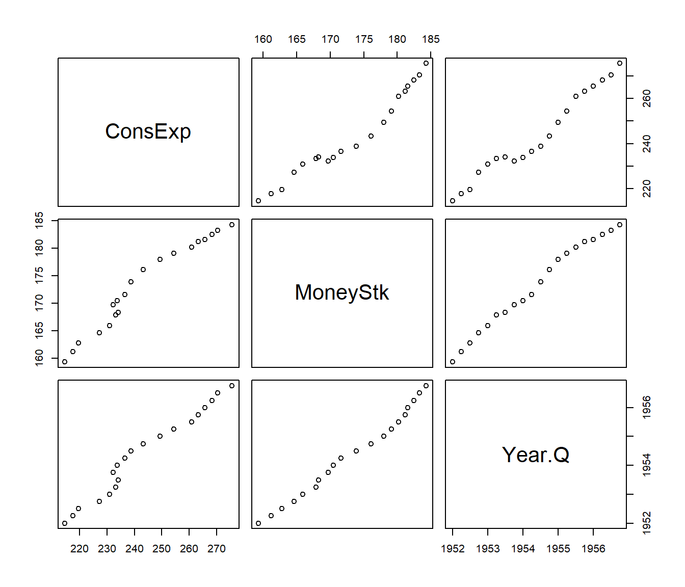
This example from the Chatterjee and Price book (3rd Ed, p202). It concerns Consumer Expenditure (y) and the Stock of Money (x) in billions of US Dollars.
A simple theoretical model suggests \[y = \alpha + \beta x + \varepsilon\]
where the so-called multiplier, \(\beta\), is a quantity of considerable importance to fiscal and monetary policy.
| Year | Quarter | ConsExp | MoneyStk | Year.Q |
|---|---|---|---|---|
| 1952 | 1 | 214.6 | 159.3 | 1952.00 |
| 1952 | 2 | 217.7 | 161.2 | 1952.25 |
| 1952 | 3 | 219.6 | 162.8 | 1952.50 |
| 1952 | 4 | 227.2 | 164.6 | 1952.75 |
| 1953 | 1 | 230.9 | 165.9 | 1953.00 |
| 1953 | 2 | 233.3 | 167.9 | 1953.25 |

A regression seems to give us quite a good estimate of \(\beta\):
Call:
lm(formula = ConsExp ~ MoneyStk, data = MoneyStock)

Residuals:
   Min     1Q Median     3Q    Max
-7.176 -3.396  1.396  2.928  6.361

Coefficients:
             Estimate Std. Error t value Pr(>|t|)
(Intercept) -154.7192    19.8500  -7.794 3.54e-07 ***
MoneyStk       2.3004     0.1146  20.080 8.99e-14 ***
---
Signif. codes:  0 '***' 0.001 '**' 0.01 '*' 0.05 '.' 0.1 ' ' 1

Residual standard error: 3.983 on 18 degrees of freedom
Multiple R-squared:  0.9573,    Adjusted R-squared:  0.9549
F-statistic: 403.2 on 1 and 18 DF,  p-value: 8.988e-14
Note the 95% Confidence Interval for \(\beta\), using standard formulae, is \(\hat\beta \pm t_{18}(0.025) se(\hat\beta)\) i.e. 2.300 \(\pm\) 2.10 \(\times\) 0.115 or 2.06 to 2.54. The model looks to be giving useful output, but are the assumptions valid?
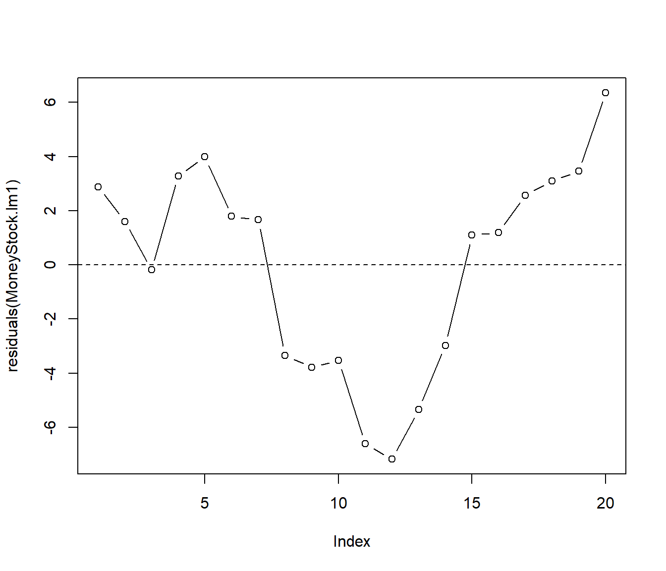
The Residual Plot above suggests problems. The residuals show the long slow wandering behaviour that is typical of positively autocorrelated data. The high positive residuals tend to be followed by more positive residuals, and high negative residuals tend to be followed by further negative ones. Thus a curve connecting the residuals together does not cross the zero line (axis) very often. The idea in the last sentence is actually the basis for our first proper test of serial correlation: the runs test.
39.4 Analysis of Runs
The residuals have signs
+ + - + + + – – – – – – – – – + + + + + + That is, there are five “runs” of residuals .
We can use the number of runs as a test for randomness. Suppose there are \(n_1\) positive residuals and \(n_2\) negative residuals.
If we assume the +s and –s occur in random order, a bit of mathematical theory can give us the expected number or runs, and also a theoretical standard deviation for the number of runs. We (or rather the computer) can compare the observed number of runs with this theoretical ideal, and come up with a P-value for the data.
Since the software will do all the calculations for us, we will not concern ourselves with the details of the method.
Then, on the basis of the P-value, we can decide whether the null hypothesis
\(H_0\): residuals are random
is indeed tenable, or whether it must be rejected. If rejected, then we conclude
\(H_1\): residuals are correlated.
An example of the calculation follows (this needs loading of the library DescTools ).
    Runs Test for Randomness

data:  residuals(MoneyStock.lm1)
runs = 5, m = 10, n = 10, p-value = 0.008985
alternative hypothesis: true number of runs is not equal the expected number
sample estimates:
median(x)
 1.395704
39.5 Durbin-Watson Test
An alternative (more powerful) approach is the Durbin-Watson test. Again this test is based on the sample residuals \(e_t\) from the linear model.
The idea is that if we have positive autocorrelation, the residual at time t will often be similar (at least in sign) to the residual at time t-1.
So if we subtract \(e_t – e_{t-1}\) then we should get a number which is small compared to the average residual. This is the basis of the test.
The actual formula for the test statistic is not examinable.
library(lmtest)
dwtest(MoneyStock.lm1, alternative = "greater")  #other alternatives are 'two.sided', 'less'
    Durbin-Watson test

data:  MoneyStock.lm1
DW = 0.32821, p-value = 2.303e-08
alternative hypothesis: true autocorrelation is greater than 0
The small P-value indicates that we reject the null hypothesis \(H_0\): no autocorrelation, in favour of the alternative hypothesis \(H_1\): positive autocorrelation.
39.6 What Can We Do About Serial Correlation?
If the series is reasonably long, then we can shift to the Time Series paradigm of analysis. This is possibly the best way.
For short series and simple regression-type problems, we can use a transformation method called the Cochrane-Orcutt method.
39.6.1 Cochrane-Orcutt method (details can be omitted 2025)
The following method can be applied to models with more than one predictor variable.
Suppose the errors in the model \[ Y_t = \alpha + \beta X_t + \varepsilon_t\]
are AR(1) i.e. a first-order autoregressive series
\[\varepsilon_t = \phi \varepsilon_{t-1} + \eta_t\]
This represents that the errors \(\varepsilon_t\) at one time point \(t\) “remember” where they were the previous time point, \(\varepsilon_{t-1}\), but then there is an additional independent error component \(\eta_t\) specific to that time point.
(Independent essentially means we can’t predict any specific component from any previous component.)
The multiplier \(\phi\) is a number between -1 and +1, that ensures that the effect of previous years gradually dies out, so that the series should eventually return to around the long-term trend. It turns out that \(\phi\) equals the autocorrelation coefficient,
\[\phi = \mbox{Corr}(Y_t, Y_{t-1}) = \mbox{Corr}( \varepsilon_t,\varepsilon_{t-1})~.\]
Now suppose we let \(y_t^*= y_t - \phi y_{t-1}\) and \(x_t^* = x_t - \phi x_{t-1}\).
Now
\[y_t^* = (\alpha + \beta X_t + \varepsilon_t) - \phi( \alpha + \beta X_{t-1} + \varepsilon_{t-1})\] \[= \alpha(1-\phi) + \beta (x_t-\phi x_{t-1}) + (\varepsilon_t - \phi \varepsilon_{t-1}) = \alpha^* + \beta^* x_t^* + \eta_t ~~~~ (*)\] where \(\alpha^* = \alpha(1-\phi)\), \(\beta^* = \beta\) and the errors \(\eta_t\) are uncorrelated, so that the model (*) satisfies the general linear model assumptions.
However \(\phi\) is not known. So we need to plug in an estimate, which we can get from Time Series Analysis or the Durbin-Watson test. We can fit the model, then, using the Cochrane-Orcutt Iterative Method. The steps are:
Calculate \(\alpha\) and \(\beta\) by ordinary least squares.
Calculate the residuals \(e_t\), and from these estimate \(\rho\).
Fit the regression model (*) by least squares, using transformed variables \(y^*\) and \(x^*\).
Estimate \(\alpha^*\) and \(\beta^*\).
- Compute residuals and examine again for autocorrelation. If there is none, then stop; if there is still autocorrelation then repeat from step 2 using residuals from step 3.
In practice Chatterjee and Price advise that if the one-step procedure doesn’t remove the autocorrelation then one should look for alternative methods, since further iteration is not likely to give much improvement.
39.6.2 Example
For the MoneyStock problem, \(r=0.751\) by the dwt output. We use this as an estimate of \(\phi\).
r = 0.751
y = MoneyStock$ConsExp
yStar = y[2:20] - r * y[1:19]
x = MoneyStock$MoneyStk
xStar = x[2:20] - r * x[1:19]
lmstar = lm(yStar ~ xStar)

dwtest(lmstar)
    Durbin-Watson test

data:  lmstar
DW = 1.427, p-value = 0.05814
alternative hypothesis: true autocorrelation is greater than 0
Call:
lm(formula = yStar ~ xStar)

Residuals:
    Min      1Q  Median      3Q     Max
-4.3746 -0.7854  0.2731  1.0405  3.9782

Coefficients:
            Estimate Std. Error t value Pr(>|t|)
(Intercept) -53.6355    13.6166  -3.939  0.00106 **
xStar         2.6440     0.3074   8.602 1.34e-07 ***
---
Signif. codes:  0 '***' 0.001 '**' 0.01 '*' 0.05 '.' 0.1 ' ' 1

Residual standard error: 2.262 on 17 degrees of freedom
Multiple R-squared:  0.8132,    Adjusted R-squared:  0.8022
F-statistic: 74 on 1 and 17 DF, p-value: 1.34e-07 2.5 % 97.5 %
(Intercept) -82.363983 -24.907052
xStar 1.995503 3.292408The transformed series has a non-significant Durbin-Watson test, so it looks that the first-order autocorrelation has been fixed.
The confidence interval for the regression coefficients show that \(\beta\) is in the wider interval (2.0, 3.29). So our real knowledge of \(\beta\) is much less precise than the earlier misleading regression model have told us.
39.6.3 Conclusion
The above example illustrates the point made earlier, that ignoring the autocorrelation can lead to misleading results.
In particular, positive autocorrelation implies that the usual (independence model) standard errors of the slopes are too small, while negative autocorrelation implies that the standard errors in the independence model are too big.