Lecture 39 Appendix: Nonlinear least squares
This topic introduces the concept of nonlinear regression models, iterative fitting by direct search, Gauss-Newton algorithm.
39.1 When the Response is a Nonlinear Function of the Regression Parameters
We consider what happens when the relationship between \(Y\) (response) and \(X\) (predictor) is known to be a particular curve that cannot be made linear by transformation.
That is, suppose \[ y = f(x) + \varepsilon\]
Where \(f(x)\) denotes some function of \(x\) (e.g. a curve), and where the error variation \(\varepsilon\) around the curve is normally distributed with constant variance as before.
Suppose we have a general idea of the shape of the curve, but the precise details depend on some unknown parameters, say \(\alpha, \beta\) and \(\gamma\).
The task, as in ordinary linear regression, reduces to that of estimating the parameters. Now in principle we can estimate \(\alpha, \beta\) and \(\gamma\) by least squares as before. That is, we simply choose those estimates that make the squared error of our curve as small as possible: i.e. the least squares problem is to minimize \[ SS_{error} = \sum \left(y_i - f(x_i; \alpha,\beta,\gamma )\right) ^2 \] or equivalently minimise the residual standard error \(S = \sqrt{SS_{error}/{(n-p)}}\).
The only difficulty or difference to the previous situation is that we do not have simple formulas to use arising out of the matrix linear algebra, as the curve \(f(x)\) is not linear in \(\alpha, \beta\) and \(\gamma\).
A couple of examples of functions \(f(x)\) that are nonlinear in the parameters are:
- Suppose
\[ f(x_i; \alpha,\beta_0,\beta_1) = \alpha~~ \frac{ e^{\beta_0+ \beta_1 x}}{ 1+e^{\beta_0+ \beta_1 x} } + \varepsilon\]
This is the so-called logistic curve, which models a phenomenon (such as sales) that goes from zero to some upper limit \(\alpha\).
(Note \(\alpha\) is an asymptote for the curve but the individual data can go randomly above or below the curve).
This model cannot be made linear, but in principle we can use any mathematical method we wish to find those estimates of \(\alpha,\beta_0\),\(\beta_1\) that minimize
\(SS_{error} = \sum (y_i - \hat y_i )^2\)
where
\[\hat y_i = \hat\alpha~~\frac{e^{\hat\beta_0+ \hat\beta_1 x} }{ 1+e^{\hat\beta_0+ \hat\beta_1 x} } ~~.\]
- A somewhat simpler example, but also nonlinear, is
\[ y_i = \beta_0 + \beta_1 x_i^{\alpha} \]
where \(\alpha\) is unknown. Again this cannot be made linear in \(\alpha,\beta_0\) and \(\beta_1\) but in this example the model fitting could be done simply by guessing \(\alpha\) and creating a new explanatory variable \(x_{new} = x^\alpha\). Then \(\beta_0\) and \(\beta_1\) can be found by linear regression of \(y\) on \(x_{new}\).
39.2 Case Study using Direct Search
The following example concerns some data on \(Y\) = the number of manhours used in surgical cases in 15 US navy hospitals, versus \(X\)= the number of cases treated.
The purpose of the analysis was to develop a preliminary manpower equation for estimation of manhours per month expended on surgical services.
   Manhours Cases
1      1275   230
2      1350   235
3      1650   250
4      2000   277
5      3750   522
6      4222   545
7      5018   625
8      6125   713
9      6200   735
10     8150   820
11     9975   992
12    12200  1322
13    12750  1900
14    13014  2022
15 13275 2155plot(Manhours ~ Cases, data = manhours)
mh1 = lm(Manhours ~ Cases, data = manhours)
abline(coef(mh1))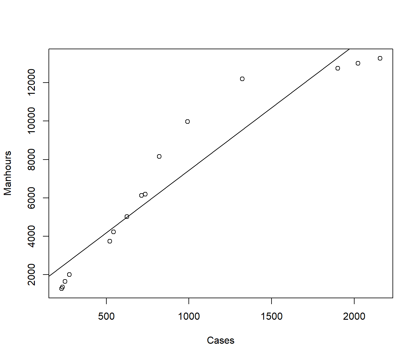
We could use trial and error. A straight-line model \(\alpha=1\) does not seem suitable. We could try a model \(\sqrt X\) (i.e. \(\alpha=0.5\)).
Call:
lm(formula = Manhours ~ Cases, data = manhours)

Residuals:
    Min      1Q  Median      3Q     Max
-1697.0 -1003.5  -561.2   510.3  2653.2

Coefficients:
            Estimate Std. Error t value Pr(>|t|)
(Intercept) 936.9261   631.4785   1.484    0.162
Cases         6.5128     0.5764  11.299 4.29e-08 ***
---
Signif. codes:  0 '***' 0.001 '**' 0.01 '*' 0.05 '.' 0.1 ' ' 1

Residual standard error: 1428 on 13 degrees of freedom
Multiple R-squared:  0.9076,    Adjusted R-squared:  0.9005
F-statistic: 127.7 on 1 and 13 DF,  p-value: 4.288e-08
Call:
lm(formula = Manhours ~ Casenew)

Residuals:
     Min       1Q   Median       3Q      Max
-1069.77  -547.39  -177.25   -65.14  2005.86

Coefficients:
            Estimate Std. Error t value Pr(>|t|)
(Intercept) -4803.30     708.57  -6.779 1.30e-05 ***
Casenew       412.48      23.76  17.362 2.25e-10 ***
---
Signif. codes:  0 '***' 0.001 '**' 0.01 '*' 0.05 '.' 0.1 ' ' 1

Residual standard error: 954.8 on 13 degrees of freedom
Multiple R-squared:  0.9587,    Adjusted R-squared:  0.9555
F-statistic: 301.4 on 1 and 13 DF,  p-value: 2.245e-10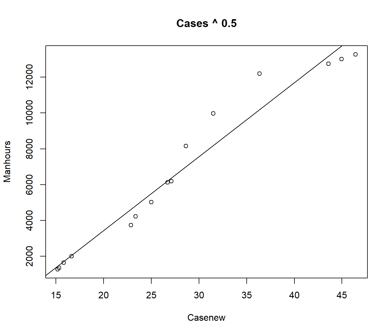
Note the residual standard error is smaller for this model. Let’s try the fourth root.
Call:
lm(formula = Manhours ~ Casenew)

Residuals:
    Min      1Q  Median      3Q     Max
-1134.3  -581.6  -184.9   309.2  1793.5

Coefficients:
            Estimate Std. Error t value Pr(>|t|)
(Intercept) -16232.1     1228.1  -13.22 6.51e-09 ***
Casenew       4417.8      232.3   19.02 7.15e-11 ***
---
Signif. codes:  0 '***' 0.001 '**' 0.01 '*' 0.05 '.' 0.1 ' ' 1

Residual standard error: 874.6 on 13 degrees of freedom
Multiple R-squared:  0.9653,    Adjusted R-squared:  0.9626
F-statistic: 361.8 on 1 and 13 DF,  p-value: 7.148e-11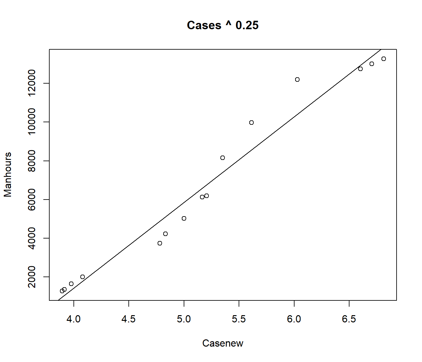
Again the residual standard error is smaller. Suppose we try a grid of values for \(\alpha\)
alpha = rse = rep(0, 10)
for (i in 1:10) {
    alpha[i] = i/10
    casenew = Cases^alpha[i]
    rse[i] = summary(lm(Manhours ~ casenew))$sigma
}
cbind(alpha, rse)
alpha rse
[1,] 0.1 920.0195
[2,] 0.2 881.7700
[3,] 0.3 875.5447
[4,] 0.4 901.2579
[5,] 0.5 954.8140
[6,] 0.6 1029.8343
[7,] 0.7 1119.6818
[8,] 0.8 1218.6620
[9,] 0.9 1322.3660
[10,] 1.0 1427.5653It looks like the minimum is for \(\alpha\) between 0.2 and 0.4
alpha = rse = rep(0, 20)
for (i in 1:20) {
    alpha[i] = 0.2 + i/100
    casenew = Cases^alpha[i]
    rse[i] = summary(lm(Manhours ~ casenew))$sigma
}
cbind(alpha, rse)
alpha rse
[1,] 0.21 879.6730
[2,] 0.22 877.9018
[3,] 0.23 876.4577
[4,] 0.24 875.3420
[5,] 0.25 874.5553
[6,] 0.26 874.0976
[7,] 0.27 873.9687
[8,] 0.28 874.1678
[9,] 0.29 874.6937
[10,] 0.30 875.5447
[11,] 0.31 876.7186
[12,] 0.32 878.2128
[13,] 0.33 880.0244
[14,] 0.34 882.1499
[15,] 0.35 884.5855
[16,] 0.36 887.3271
[17,] 0.37 890.3701
[18,] 0.38 893.7098
[19,] 0.39 897.3409
[20,] 0.40 901.2579It looks like the minimum is for \(\alpha\) between 0.26 and 0.28.
alpha = rse = rep(0, 20)
for (i in 1:20) {
    alpha[i] = 0.26 + i/1000
    casenew = Cases^alpha[i]
    rse[i] = summary(lm(Manhours ~ casenew))$sigma
}
cbind(alpha, rse)
alpha rse
[1,] 0.261 874.0699
[2,] 0.262 874.0455
[3,] 0.263 874.0244
[4,] 0.264 874.0066
[5,] 0.265 873.9921
[6,] 0.266 873.9809
[7,] 0.267 873.9729
[8,] 0.268 873.9682
[9,] 0.269 873.9668
[10,] 0.270 873.9687
[11,] 0.271 873.9739
[12,] 0.272 873.9823
[13,] 0.273 873.9941
[14,] 0.274 874.0091
[15,] 0.275 874.0273
[16,] 0.276 874.0489
[17,] 0.277 874.0737
[18,] 0.278 874.1018
[19,] 0.279 874.1332
[20,] 0.280 874.1678It looks like the minimum \(S\) is obtained for \(\alpha \approx 0.269\). The procedure could be repeated to obtain the minimum RSE to more significant figures but, in view of the small changes we are achieving, little will be achieved by going further.
Call:
lm(formula = Manhours ~ casenew)

Residuals:
    Min      1Q  Median      3Q     Max
-1111.6  -586.3  -207.4   278.2  1806.2

Coefficients:
            Estimate Std. Error t value Pr(>|t|)
(Intercept) -14619.7     1144.1  -12.78 9.80e-09 ***
casenew       3618.8      190.1   19.03 7.09e-11 ***
---
Signif. codes:  0 '***' 0.001 '**' 0.01 '*' 0.05 '.' 0.1 ' ' 1

Residual standard error: 874 on 13 degrees of freedom
Multiple R-squared:  0.9654,    Adjusted R-squared:  0.9627
F-statistic: 362.3 on 1 and 13 DF,  p-value: 7.086e-11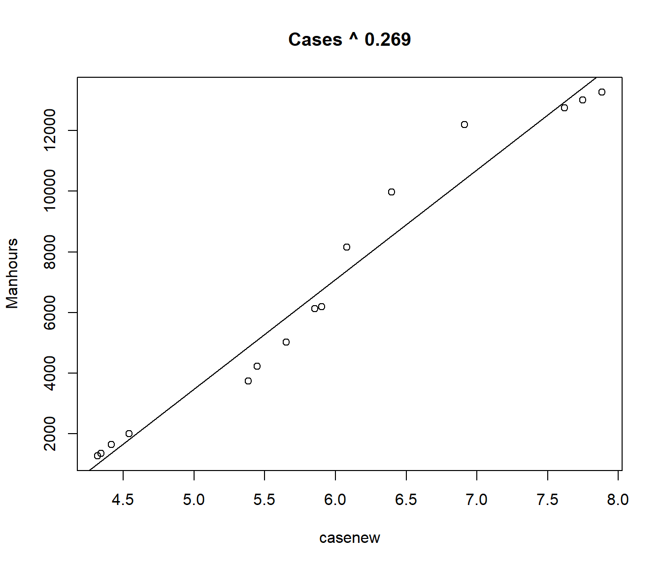
39.3 The Gauss-Newton Algorithm
The alternative to using direct search is to use a mathematical technique such as the Gauss-Newton Algorithm .
The idea of the algorithm is to approximate the curve \(f(x_i; \alpha,\beta,\gamma)\) by a sum of straight lines involving \(\alpha,\beta\) and \(\gamma\). That is, a linearized approximation to the curve.
The mathematical ideas are in an word document on Stream, but are not examinable.
The main points are:
The process of model-fitting is iterative. That is, it involves a series of repeated linear regressions with slightly different data each time, converging to a fixed answer as we get closer and closer to the optimal estimates.
The Gauss-Newton method is guaranteed to converge quickly to the optimal estimates, provided that our initial starting point is close enough.
The method also produces approximate hypothesis tests and confidence intervals.
The nls() nonlinear least squares procedure implements the Gauss-Newton algorithm.
We need to specify the formula, and (preferably) reasonable starting values.
manhours.nls = nls(Manhours ~ beta0 + beta1 * (Cases^alpha), start = list(alpha = 0.25,
    beta0 = -16000, beta1 = 4400), data = manhours)

summary(manhours.nls)
Formula: Manhours ~ beta0 + beta1 * (Cases^alpha)

Parameters:
        Estimate Std. Error t value Pr(>|t|)
alpha  2.689e-01  1.585e-01   1.697    0.115
beta0 -1.463e+04  1.256e+04  -1.164    0.267
beta1  3.622e+03  5.954e+03   0.608    0.554

Residual standard error: 909.7 on 12 degrees of freedom

Number of iterations to convergence: 6
Achieved convergence tolerance: 2.462e-06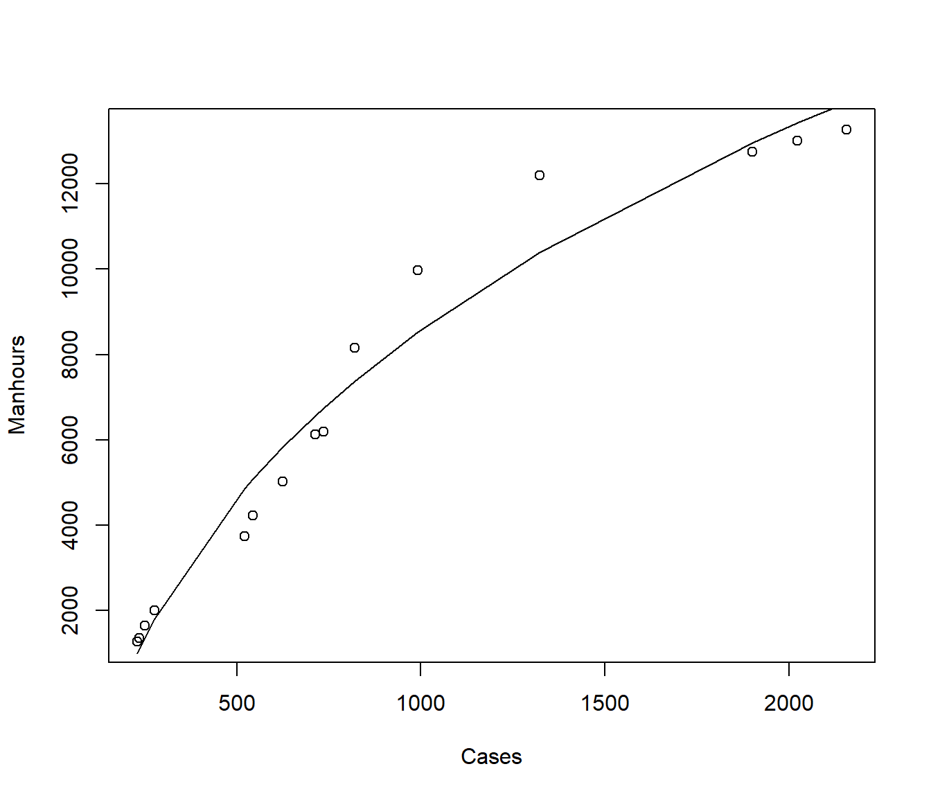
We can calculate an approximate confidence interval for \(\alpha\) using \[ \hat\alpha \pm t_{n-p}(0.025)*SE(\hat\alpha)\]
           Estimate   Std. Error    t value  Pr(>|t|)
alpha  2.689232e-01     0.158476  1.6969329 0.1154707
beta0 -1.462572e+04 12564.190279 -1.1640799 0.2670141
beta1  3.621670e+03  5954.344902  0.6082398 0.5543666
est = summary(manhours.nls)$coefficients[1]
se = summary(manhours.nls)$coefficients[4]
lower = est + qt(0.025, df = 15 - 3) * se
upper = est + qt(0.975, df = 15 - 3) * se
cbind(est, se, lower, upper) est se lower upper
[1,] 0.2689232 0.158476 -0.07636641 0.6142128We can conclude from this that we could not reject a hypothesis that \(\alpha\) equalled any value between -0.07 and 0.6.
In particular, we could have stuck with the square-root transformation (\(\alpha=0.5\)) or used the log transformation (recall this takes the place of \(\alpha=0\) in the ladder of powers).
39.4 Example: A Growth Curve Model with an Maximum
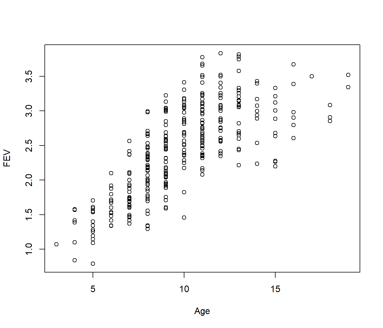
Recall the fev data relating forced expiration volume (FEV) to girls’ ages. This seemed to flatten off after about age 10.
We will model the growth using a logistic curve with unknown maximum.
\[ f(x_i; \alpha,\beta_0,\beta_1) = \alpha~~\frac{e^{\beta_0+ \beta_1 x}}{ 1+e^{\beta_0+ \beta_1 x} } + \varepsilon\]
From the graph the maximum \(\alpha \approx 3\), so setting
\[FEV \approx 3 ~~\frac{e^{\beta_0 + \beta_1 Age}}{ 1+ e^{\beta_0 + \beta_1 Age}}\]
we can rearrange this as
\[1+ e^{\beta_0 + \beta_1 Age} \approx \frac{3}{FEV} ~ e^{\beta_0 + \beta_1 Age} \]
Gather up the \(e^{\beta_0 + \beta_1 Age}\) terms
\[ \frac{1}{3/FEV - 1} \approx e^{\beta_0 + \beta_1 Age}\] and then if we take logs we can use the left-hand side as the “response” in a regression
\[ Y_{new} = \log\left(\frac{1}{3/FEV - 1}\right)\approx \beta_0 + \beta_1 Age \] to give us starting values for \(\beta_0\) and \(\beta_1\):
Warning in log(3/FEV - 1): NaNs produced
Call:
lm(formula = -log(3/FEV - 1) ~ Age)

Residuals:
    Min      1Q  Median      3Q     Max
-1.9603 -0.5223 -0.1590  0.2990  5.0842

Coefficients:
            Estimate Std. Error t value Pr(>|t|)
(Intercept) -1.30548    0.21129  -6.179 2.78e-09 ***
Age          0.28493    0.02226  12.799  < 2e-16 ***
---
Signif. codes:  0 '***' 0.001 '**' 0.01 '*' 0.05 '.' 0.1 ' ' 1

Residual standard error: 0.9443 on 238 degrees of freedom
  (78 observations deleted due to missingness)
Multiple R-squared:  0.4077,    Adjusted R-squared:  0.4052
F-statistic: 163.8 on 1 and 238 DF,  p-value: < 2.2e-16
So we will use starting values \(\alpha=3\), \(\beta_0= -1.3\) and \(\beta_1=0.28\)
fev.nls = nls(FEV ~ alpha * exp(beta0 + beta1 * Age)/(1 + exp(beta0 + beta1 * Age)),
    start = list(alpha = 3, beta0 = -1.3, beta1 = 0.28))
summary(fev.nls)
Formula: FEV ~ alpha * exp(beta0 + beta1 * Age)/(1 + exp(beta0 + beta1 *
    Age))

Parameters:
      Estimate Std. Error t value Pr(>|t|)
alpha  3.21164    0.08682   36.99   <2e-16 ***
beta0 -2.16822    0.21482  -10.09   <2e-16 ***
beta1  0.36561    0.03620   10.10   <2e-16 ***
---
Signif. codes:  0 '***' 0.001 '**' 0.01 '*' 0.05 '.' 0.1 ' ' 1

Residual standard error: 0.3956 on 315 degrees of freedom

Number of iterations to convergence: 5
Achieved convergence tolerance: 6.266e-06plot(FEV ~ Age)
lines(30:200/10, predict(fev.nls, newdata = data.frame(Age = 30:200/10)), lty = 1,
col = 2, lwd = 3)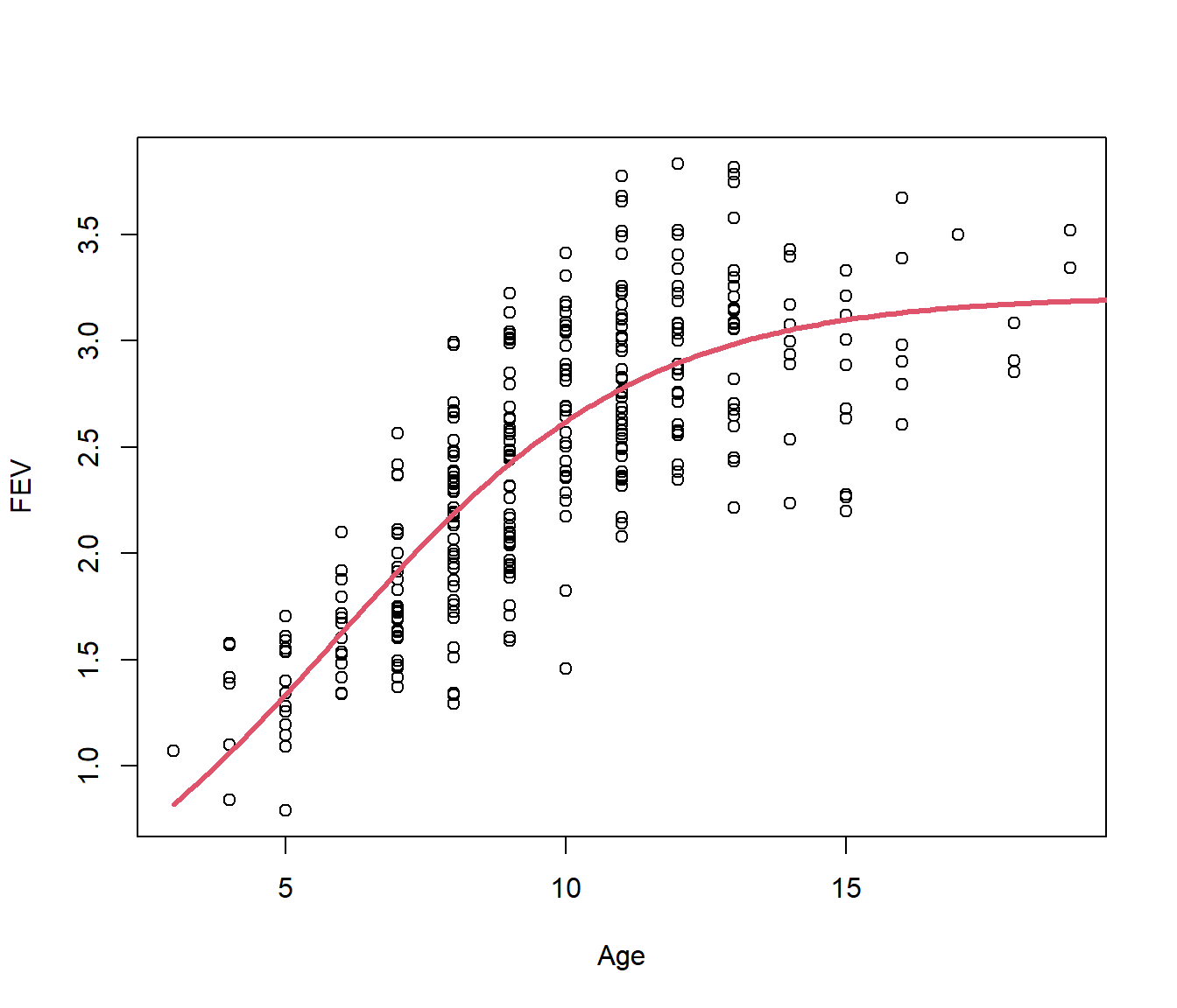
This has converged. Note the residual standard error is 0.3956, which is slightly bigger than for the piecewise model looked at earlier (S=0.39) but the curve seems more reasonable than having a sharp corner.
We can get a slightly better fit by adding a quadratic term in Age. In the following we use starting value \(\beta_2=0\).
fev.nls2 = nls(FEV ~ alpha * exp(beta0 + beta1 * Age + beta2 * Age^2)/(1 + exp(beta0 +
    beta1 * Age + beta2 * Age^2)), start = list(alpha = 3, beta0 = -1.3, beta1 = 0.28,
    beta2 = 0), data = fev)
summary(fev.nls2)
Formula: FEV ~ alpha * exp(beta0 + beta1 * Age + beta2 * Age^2)/(1 + exp(beta0 +
    beta1 * Age + beta2 * Age^2))

Parameters:
      Estimate Std. Error t value Pr(>|t|)
alpha  3.03273    0.05788  52.393  < 2e-16 ***
beta0 -0.06772    0.75358  -0.090  0.92846
beta1 -0.23896    0.21936  -1.089  0.27684
beta2  0.04437    0.01619   2.741  0.00647 **
---
Signif. codes:  0 '***' 0.001 '**' 0.01 '*' 0.05 '.' 0.1 ' ' 1

Residual standard error: 0.3906 on 314 degrees of freedom

Number of iterations to convergence: 7
Achieved convergence tolerance: 2.889e-06plot(FEV ~ Age)
lines(30:200/10, predict(fev.nls2, newdata = data.frame(Age = 30:200/10)), lty = 1,
col = 2, lwd = 3)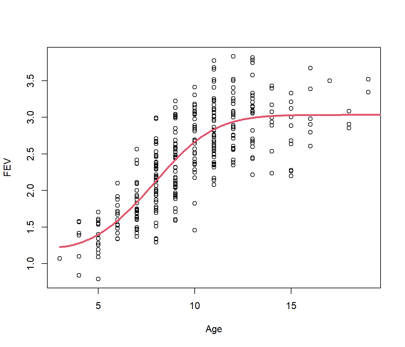
39.5 Piecewise Regression with an Unknown Knot
Recall that sometimes we wish to fit a piecewise regression model, but the location of the knot is unknown.
This then is becomes a nonlinear regression model, with the location of the knot taking the role of the alpha parameter above (not meaning that it enters the equation the same way, but that if the knot is known, then every other parameter can be fitted by linear regression).
Strictly speaking the Gauss-Newton algorithm does not quite work, as the knot gives a ‘corner’ to the lines, or even a jump in the level of the lines, and this means that the calculus on which the method was originally based breaks down. However the nls() routine can be made to cope.
39.5.1 Nonlinear regression for a change-slope model: the Thai Baht.
The data here refer to the Thai Baht Exchange Rate \(Y\) vs Time (time measured in hundreds of days, hDays. ) The graph below shows \(Y\) vs hDays with a cubic model. The model looks like it would be unsafe for extrapolation on the right.
## baht = read.csv("baht.csv", header = TRUE)

Y = baht$Y
hDays = baht$hDays

plot(Y ~ hDays)
cubic = lm(Y ~ poly(hDays, 3))
summary(cubic)$sigma
[1] 0.008618117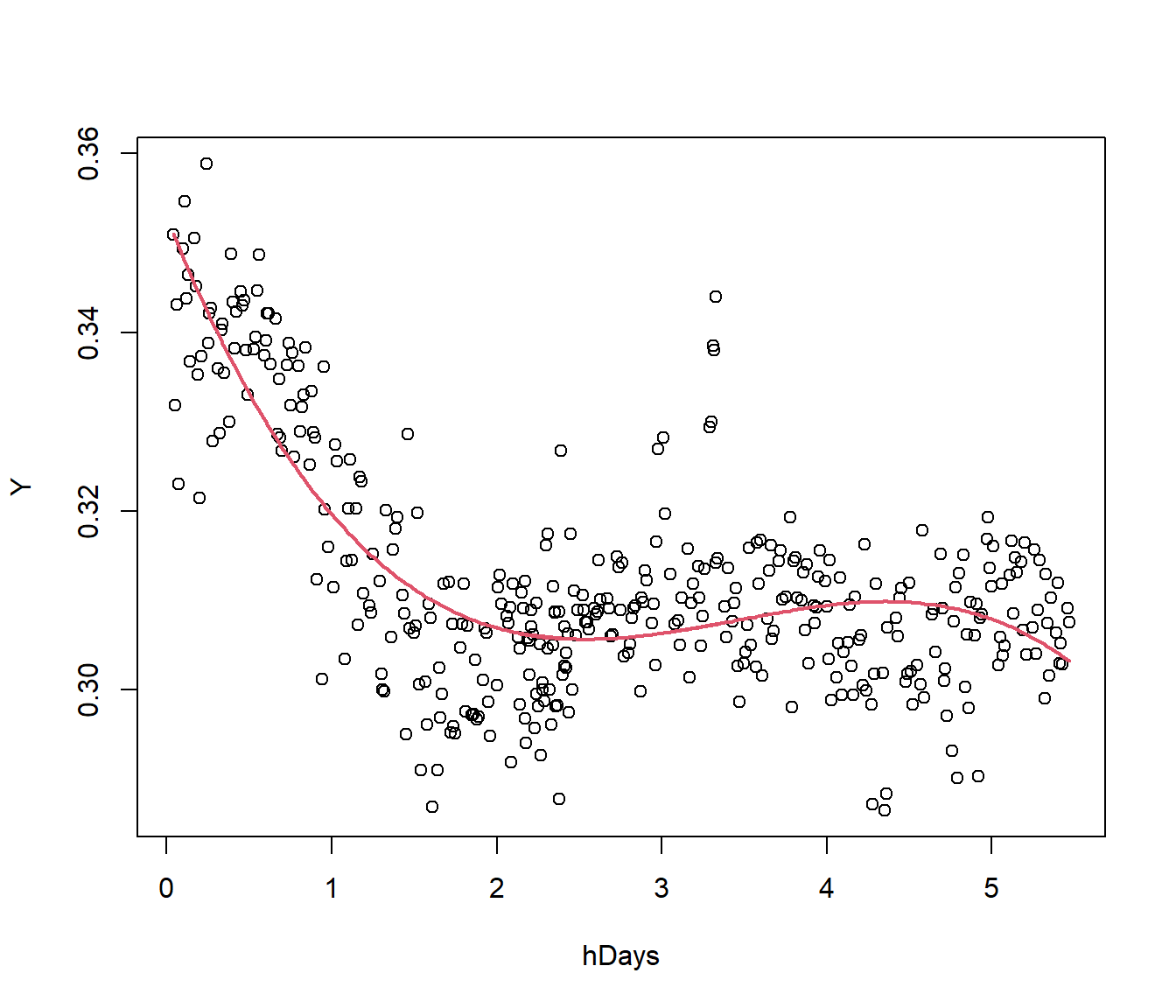
We consider a piecewise model \[ Y = \beta_0 + \beta_1. hDays + \beta_2 (hDays-k)_+ \] where \(k\) is unknown but probably near 2. We will use this guess to give starting values for the other parameters.
Call:
lm(formula = Y ~ hDays + I((abs(hDays - 2) + hDays - 2)/2))

Residuals:
      Min        1Q    Median        3Q       Max
-0.024944 -0.005216  0.001020  0.004923  0.037731

Coefficients:
                                    Estimate Std. Error t value Pr(>|t|)
(Intercept)                        0.3443525  0.0013566  253.84   <2e-16 ***
hDays                             -0.0201913  0.0008924  -22.63   <2e-16 ***
I((abs(hDays - 2) + hDays - 2)/2)  0.0219204  0.0012007   18.26   <2e-16 ***
---
Signif. codes:  0 '***' 0.001 '**' 0.01 '*' 0.05 '.' 0.1 ' ' 1

Residual standard error: 0.008564 on 386 degrees of freedom
Multiple R-squared:  0.6141,    Adjusted R-squared:  0.6121
F-statistic: 307.2 on 2 and 386 DF,  p-value: < 2.2e-16
This gives starting estimates \(\beta_0\approx 0.34, ~~ \beta_1 \approx -0.02,~~ \beta_2 \approx 0.022, ~~k=2\).
The following code fits the model, but some iteration control parameters were needed, presumably because of the corner. (Other statistical software such as SPSS and Minitab have less problems fitting this model.)
baht.nls = nls(Y ~ beta0 + beta1 * hDays + beta2 * I((abs(hDays - k) + hDays - k)/2),
    start = list(beta0 = 0.34, beta1 = -0.02, beta2 = 0.022, k = 2), data = baht,
    nls.control(warnOnly = TRUE, minFactor = 1/2048))
Warning in nls(Y ~ beta0 + beta1 * hDays + beta2 * I((abs(hDays - k) + hDays -
: step factor 0.000244141 reduced below 'minFactor' of 0.000488281
Formula: Y ~ beta0 + beta1 * hDays + beta2 * I((abs(hDays - k) + hDays -
    k)/2)

Parameters:
       Estimate Std. Error t value Pr(>|t|)
beta0  0.349459   0.001597  218.88   <2e-16 ***
beta1 -0.027767   0.001772  -15.67   <2e-16 ***
beta2  0.028657   0.001821   15.73   <2e-16 ***
k      1.579995   0.064909   24.34   <2e-16 ***
---
Signif. codes:  0 '***' 0.001 '**' 0.01 '*' 0.05 '.' 0.1 ' ' 1

Residual standard error: 0.008074 on 385 degrees of freedom

Number of iterations till stop: 14
Achieved convergence tolerance: 0.008517
Reason stopped: step factor 0.000244141 reduced below 'minFactor' of 0.000488281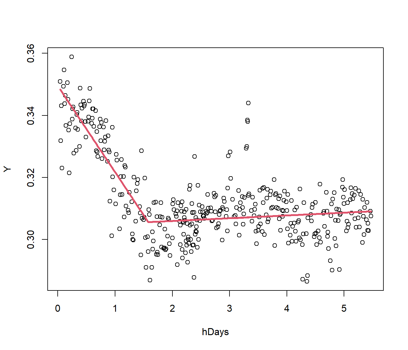
The graph seems much more reasonable. Note it changed the \(k\) to 1.57.
In terms of residual standard error, which is the better-fitting model, the cubic or the change-point model? (From above the cubic graph S =0.008618).
39.2.1 Comments on direct search
Direct searching on a grid may get to a solution, but the method has disadvantages.
It is time-consuming, requiring programming and/or human intervention.
If we have several parameters to search for, we may have to use a grid in two, three or more dimensions, which is computationally intensive.
Even once we get to a point estimate, we do not have a standard error for the estimate, so we do not know really how accurate it is. We cannot compute confidence intervals or hypothesis tests regarding the parameters.
We now consider a more convenient method that overcomes all these handicaps.