Lecture 3 Simple Linear Regression
As we have seen, simple linear regression seeks to model the relationship between the mean of the response y and a single predictor x.
You will have met simple linear regression in other statistics courses, so some of the material in this lecture should be revision.
Nonetheless, simple linear regression provides a friendly context to introduce notation, remind you of fundamental concepts, and take a first look at statistical modelling with R.
3.1 Pulse and Height
The following R code
- reads the pulse data into R (from a text file); and then
- prints out the first few rows of the data for simple viewing.
## PulseData <- read.csv(file = "https://r-resources.massey.ac.nz/data/161251/pulse.csv",
##     header = TRUE)
head(PulseData)
Height Pulse
1 160 68
2 167 80
3 162 84
4 175 80
5 177 80
6 185 80- We would normally then look at some plots. Only one scatter plot is possible. We could display it using either a simple
plot(), or a more fancyggplot(), but it is essentially the same graph. You could compare the results of the old base graphics style:
with the more modern ggplot2 style:
library(ggplot2)
PulseData |>
    ggplot(mapping = aes(x = Height, y = Pulse)) + geom_point() + ylab("Resting pulse rate (beats per minute)") +
    xlab("Height (in centimeters) ")
Figure 3.1: Plot of resting pulse rate (beats per minute) versus height (in centimeters) for a sample of 50 hospital patients. Source: A Handbook of Small Data Sets by Hand, Daly, Lunn, McConway and Ostrowski.
The choice is yours; you need to choose what is best for your audience. If your audience is just you, then do what you find easier. If you’re wanting to look good when you’re delivering presentations, then you’ll benefit from getting to grips with the ggplot() way of working.
It is of interest to know whether pulse rate is truly dependent on height.
View pulse as response (y) variable and height as predictor (x) variable.
We can formally test whether this really is the case by using a simple linear regression model.
Note there is one observation (patient resting pulse 116) which is distant from the main bulk of data.
3.2 Basics of Simple Linear Regression: Data
Quantitative data occur in pairs: (x1,y1), …,(xn,yn).
yi denotes the response variable and xi the explanatory variable for the ith individual.
The aim is to estimate the mean response for any given value of the explanatory variable.
It therefore makes sense to think of x1,…,xn as fixed constants, while y1, …, yn are chance values taken by random variables Y1,…, Yn.
3.3 Basics of Simple Linear Regression: Model
Now recall that The linear regression model is
\[Y_i = \beta_0 + \beta_1 x_i + \varepsilon_i\]
where
- \(\beta_0, \beta_1\) are regression parameters.
- \(\varepsilon_1, \ldots ,\varepsilon_n\) are error terms, about which we make the following assumptions.
A1. The expected value of the errors \(E[\varepsilon_i] = 0\) for i=1,…,n.
A2. The errors \(\varepsilon_1, \ldots ,\varepsilon_n\) are independent. N.B. A2 might be new to you. Near the end of the course we will consider what happens if this assumption is wrong.
A3. The error variance \(\mbox{var}(\varepsilon_i) = \sigma^2\) (an unknown constant) for i=1,…,n.
A4. The errors \(\varepsilon_1, \ldots ,\varepsilon_n\) are normally distributed.
N.B. We refer back to these four assumptions many times in this course; they will often be referred to using the shorthand A1 to A4.
The validity of the simple regression model given above and Assumption A1 implies that
\[E[Y_i] = \mu_i = \beta_0 + \beta_1 x_i\]
So we say that \(E[Y_i] = \mu_i\) is the expected value of Yi given (or conditional upon) xi.
3.4 Parameter Estimation
How do we estimate the parameters \(\beta_0\) and \(\beta_1\)?
The simplest method, which is optimal if the assumptions A1-A4 are correct, is to use the method of least squares.
Least squares estimates (LSEs) \(\hat{\beta_0}\) and \(\hat{\beta_1}\), are those values that minimize the sum of squares
\[\begin{aligned} SS(\beta_0, \beta_1) &=& \sum_{i=1}^n (y_i - \mu_i)^2\\ &=& \sum_{i=1}^n (y_i - \beta_0 - \beta_1 x_i)^2. \end{aligned}\]
It can be shown (using calculus) that \(\hat{\beta_0}\) and \(\hat{\beta_1}\) are given by
\[\hat{\beta_1} = \frac{s_{xy}}{s_{xx}}\] where
\(s_{xy} = \sum_{i=1}^n (x_i - \bar x)(y_i - \bar y)\);
\(s_{xx} = \sum_{i=1}^n (x_i - \bar x)^2\);
and \(\hat{\beta_0} = \bar y - \hat{\beta_1} \bar x \; .\)
The last formula implies that the least squares regression line goes through the centroid \(\left(\bar x, \bar y \right)\) of the data.
3.5 Properties of LSEs
Some maths shows sampling distributions of \(\hat{\beta_0}\) and \(\hat{\beta_1}\) are:
\[\hat{\beta_1} \sim N \left(\beta_1, \frac{\sigma^2}{s_{xx}} \right )\] and \[\hat{\beta_0} \sim N \left(\beta_0 , \, \sigma^2\left[\frac{1}{n} + \frac{\bar x^2}{s_{xx}}\right ] \right ) \; .\]
The details of the above formulas are not important. The practical point of the formulas is that
- the estimates are unbiased (centred on the right thing). This implies that random sampling should give you about the right answer (at least if we have a big enough dataset), and
- the estimates are normally distributed, which means we can calculate confidence intervals and hypothesis tests for \(\beta_0\) and \(\beta_1\).
The variance terms (second term within each of the N( , ) formulae) are given for completeness of your notes, but are not something we will need to calculate ourselves.
3.5.1 Class discussion
what do these sampling distributions tell us?
Just for illustration, let’s say that the model fitted to the population of data is \(Y_i = 1 + 2 x_i + \varepsilon_i\) (i=1,2,…,n) with \(\varepsilon \sim N(0,2^2)\)
To make our calculations a simpler task, let’s also say that the covariate Information we need is: Sample size n = 32, \(\bar{x} = \sqrt{2}\), and sxx = 64.
3.5.3 Answer to (i):
We are looking for \(P(\hat{\beta_1} > 3)\)
We know that the parameter is normally distributed so we will use the standard normal distribution to find the probability. Note that \(Z \sim N(0,1)\)
After inserting the values given above, this is equal to \(P \left ( Z > \frac{3 - \beta_1}{(\sigma/\sqrt{s_{xx}}) } \right )\)
Simplifying gives \(P \left ( Z > \frac{3 - 2}{(2/\sqrt{64}) } \right ) = P \left ( Z > \frac{1}{2/8} \right ) = P(Z > 4)\)
which is approximately zero.
3.6 Estimating the Error Variance
In practice, we are almost certainly working with sample data, which means the error variance, \(\sigma^2\) is also an unknown parameter.
It is important to estimate it because its square root \(\sigma\) gives us information about the natural variation in the data i.e. about how far away the individual datapoints \(Y_i\) typically are from the central line \(E[Y] =\beta_0 + \beta_1 x\).
It can be estimated using the residual sum of squares (RSS), defined by
\[RSS = \sum_{i=1}^n (y_i - \hat{\mu_i})^2 = \sum_{i=1}^n (y_i - \hat{\beta_0} - \hat{\beta_1} x_i )^2 \; .\]
where \(\hat{\mu_i} = \hat{\beta_0} + \hat{\beta_1} x_i\) is the ith fitted value; \(e_i = y_i - \hat{\mu_i}\) is the ith residual.
Then an estimate of \(\sigma^2\) is given by
\[s^2 = \frac{1}{n-2} RSS.\]
N.B. We almost always use the notation \(\hat y_i\) instead of \(\hat{\mu_i}\), but don’t lose sight of the fact that we are estimating an average even if that average is changing according to the value of a predictor.
3.7 Revised Sampling Distributions
We have seen the term \(\sigma^2\) in a number of equations. This is not known, but must be estimated from our data. When we do not know this “true” variance, we use an estimate or “sample variance” instead. This means we must alter the sampling distribution too. This happened when you used sample data to find an interval estimate of the population mean or conducted a one sample test about the population mean.
Standardizing the normal sampling distribution of \(\hat{\beta_1}\) gives
\[\frac{\hat{\beta_1} - \beta_1}{\sigma/\sqrt{s_{xx}}} \sim N(0,1)\]
Replacing \(\sigma^2\) with the estimate s2 changes the sampling distribution of \(\hat{\beta_1}\):
\[\frac{\hat{\beta_1} - \beta_1}{SE(\hat{\beta_1})} \sim t(n-2)\]
where
- the notation t(n-2) or sometimes tn-2 signifies a t-distribution with (n-2) degrees of freedom (df)
- the term \(SE(\hat{\beta_1}) = \frac{s}{\sqrt{s_{xx}}}\) is the standard error of \(\hat{\beta_1}\); i.e. the (estimated) standard deviation of the sampling distribution of \(\hat{\beta_1}\).
The sampling distribution for \(\hat{\beta_1}\) forms the basis for testing hypotheses and constructing confidence intervals for \(\beta_1\).
For testing H0: \(\beta_1 = \beta_1^0\), against H1: \(\beta_1 \ne \beta_1^0\), use the test statistic
\[t = \frac{\hat{\beta_1} - \beta_1^0}{SE(\hat{\beta_1})}.\]
We find p-value corresponding to t. As usual, smaller P indicates more evidence against H0.
A \(100(1-\alpha)\%\) confidence interval for \(\beta_1\) is
\[\left (\hat{\beta_1} - t_{\alpha/2}(n-2) SE(\hat{\beta_1}), \, \hat{\beta_1} + t_{\alpha/2}(n-2) SE(\hat{\beta_1}) \right ) .\]
3.8 The t distribution
The t distribution is used for small samples when we do not know the population variance.
You’ll see that we still use the t distribution when samples are so large that it doesn’t actually matter. Why doesn’t it matter? Because the t distribution gets closer and closer to the normal distribution as the sample size increases.
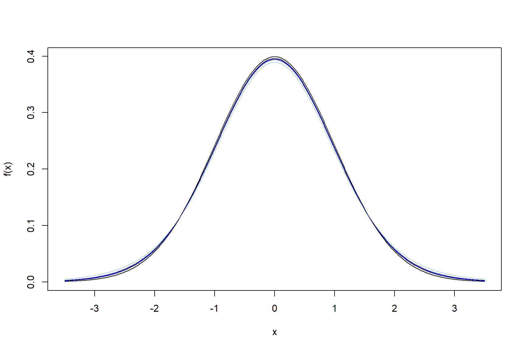
Figure 3.2: Probability density functions for t distributions; As df =10,20,30, (light to dark blue), the curves get closer to the normal curve (black)
The “fatter” tails of the t distribution mean that the critical values we use in confidence intervals are larger for smaller sample sizes.
3.9 Back to the example
For the pulse and height data, it can be shown that the fitted regression line (i.e. the regression line with least squares estimates in place of the unknown model parameters) is
\[E[\mbox{Pulse}] = 46.907 + 0.2098~\mbox{Height}\]
- Hence \(\hat{\beta_1} = 0.2098\).
Also, it can be shown that \(SE(\hat{\beta_1}) = 0.1354\).
Finally, recall that n=50.
Question: Do the data provide evidence the pulse rate depends on height?
Solution: To answer this question, we will test
H0: \(\beta_1 = 0\), versus
H1: \(\beta_1 \ne 0\)
The test statistic is
\[t = \frac{\hat{\beta_1} - \beta_1^0}{SE(\hat{\beta_1})} = \frac{0.2098}{0.1354} = 1.549\]
The (2-sided) P-value is \(P=P(|T| > 1.549) = 2 \times P(T > 1.549) = 2 \times 0.06398 = 0.128\), so we conclude that the data provide no evidence of a (simple linear) relationship between pulse rate and height.