Lecture 36 Appendix: Regression through the origin
In this material, we consider the special case of \(\beta_0=0\) (called regression through the origin).
36.1 What is regression through the origin?
Regression through the origin \((x,y)=(0,0)\) is not common but does happen. For example we consider a model where we may have a strong prior belief that there is no possibility that the intercept can be anything other than zero. Then our model reduces to \[ Y_i = \beta_1 x_i + \varepsilon_i\]
This model forces the mean value of y to equal 0 if \(x=0\). This is called regression through the origin.
All statistical packages allow you to fit this model, and it is useful at times - but one must interpret the results with care. One aspect of this warning is that we cannot use \(R^2\) to compare the goodness of fit with that of the usual linear model \(\beta_0+ \beta_1 x\).
The reason is that the usual \[R^2 = 1- \frac{\sum\left(y - \hat y\right)^2}{\sum\left(y - \bar y\right)^2}\]
refers to the improvement in fit relative to a flat line: the denominator is based on deviations around the mean. In the case of regression through the origin, the flat line would have to be the flat line going though y=0.
\[ \mbox{Fake }R^2 = 1- \frac{\sum\left(y - \hat y\right)^2}{\sum\left(y - 0\right)^2}\]
For this reason the \(R^2\) can only be used to compare two models both of the same sort, i.e. both regression through the origin or both not through the origin.
36.1.1 Manawatu wind speeds example
As an example, the dataset TenMinuteWinds.csv gives the wind speed at a Manawatu Wind Farm, every 10 minutes for one day. Wind Farms want to be able to predict the wind 10 minutes ahead, because they have to nominate in advance how much electricity they can supply to the national power grid, and there is a financial incentive for getting their prediction as close to the true amount as possible.
Download TenMinuteWinds.csv to replicate the following examples.
  Hour Minutes Speed TenMinEarlier
1    0       0  8.73          8.74
2    0      10  9.28          8.73
3    0      20  9.35          9.28
4    0      30  9.91          9.35
5    0      40  9.21          9.91
6 0 50 9.63 9.21 Hour Minutes Speed TenMinEarlier
139 23 0 10.42 9.75
140 23 10 10.38 10.42
141 23 20 8.97 10.38
142 23 30 7.97 8.97
143 23 40 8.18 7.97
144 23 50 9.23 8.18plot(Speed ~ TenMinEarlier, data = Winds)
Wind.lm = lm(Speed ~ TenMinEarlier, data = Winds)
abline(Wind.lm)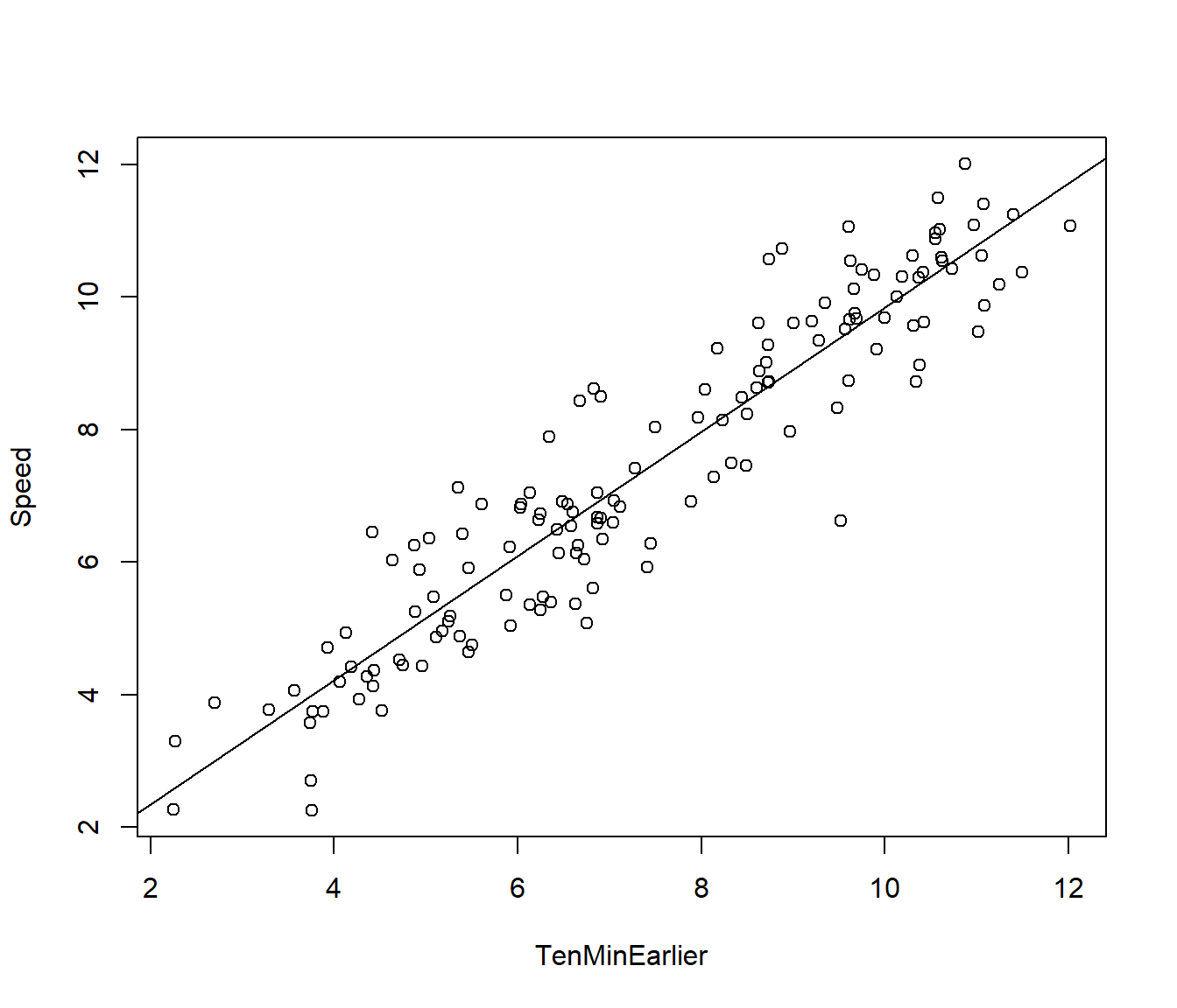
A simple model used in Industry is the so-called Persistence model \[Speed_t = Speed_{t-1} + \varepsilon_t \] where \(Speed_{t-1}\) is the wind speed 1 unit of time (one row) earlier (i.e. 10 minutes earlier .) Note the slope of this model is 1, and the intercept is 0, implying that we predict the next wind speed to be exactly the same as the last one, which seems reasonable. The intercept =0 would imply that if there is no wind 10 minutes earlier then we predict no wind next time.
Having an intercept suggests the wind speed is always increasing by that amount (on average) over time. This might be reasonable in very short runs of data, but it is not realistic for a natural system that has an equilibrium.
We can examine this model by fitting the slightly more general model
\[ Speed_t = \beta_1 Speed_{t-1} +\varepsilon_t\] and checking whether the hypothesis \(H_0: \beta_1= 1\) is reasonable.
We fit this model in R using 0 + in the model formulation
Call:
lm(formula = Speed ~ 0 + TenMinEarlier, data = Winds)

Residuals:
     Min       1Q   Median       3Q      Max
-2.83822 -0.48117  0.02208  0.51050  2.05404

Coefficients:
              Estimate Std. Error t value Pr(>|t|)
TenMinEarlier 0.994561   0.009108   109.2   <2e-16 ***
---
Signif. codes:  0 '***' 0.001 '**' 0.01 '*' 0.05 '.' 0.1 ' ' 1

Residual standard error: 0.8488 on 143 degrees of freedom
Multiple R-squared:  0.9882,    Adjusted R-squared:  0.9881
F-statistic: 1.192e+04 on 1 and 143 DF, p-value: < 2.2e-16 2.5 % 97.5 %
TenMinEarlier 0.9765582 1.012564The confidence interval shows that \(\beta_1= 1\) is included in the interval. So this indicates 1 is a plausible slope that cannot be rejected. If we want an actual p-value for \(H_0: \beta_1= 1\) vs \(H_1: \beta_1 \ne 1\) then we have to calculate our own \(T\) ratio \[ T = \frac{\hat\beta_1 -1}{se(\hat\beta_1)} \sim t_{n-1} \]
               Estimate  Std. Error  t value      Pr(>|t|)
TenMinEarlier 0.9945612 0.009107649 109.2006 1.248051e-139[1] -0.5971713[1] 1 143 1[1] 0.4486626Note that the \(df = n-1\) this time, since we are only estimating one coefficient \(\beta_1\) and not two coefficients.
However the question remains whether the assumption \(\beta_0 = 0\) is valid or not. We can examine this by comparing the output to the model with an intercept.
Call:
lm(formula = Speed ~ TenMinEarlier, data = Winds)

Residuals:
     Min       1Q   Median       3Q      Max
-2.76044 -0.56069  0.06546  0.55033  1.93953

Coefficients:
              Estimate Std. Error t value Pr(>|t|)
(Intercept)    0.46593    0.22868   2.037   0.0435 *
TenMinEarlier  0.93745    0.02944  31.839   <2e-16 ***
---
Signif. codes:  0 '***' 0.001 '**' 0.01 '*' 0.05 '.' 0.1 ' ' 1

Residual standard error: 0.8396 on 142 degrees of freedom
Multiple R-squared:  0.8771,    Adjusted R-squared:  0.8763
F-statistic:  1014 on 1 and 142 DF,  p-value: < 2.2e-16
Comparing these two models, we see that we would reject the null hypothesis \(H_0 : \beta_0 = 0\) with a p-value of 0.0435.
Also the residual standard error is lower in the model with an intercept.
What we cannot do is compare the \(R^2\) here to the Fake \(R^2\) from the model without an intercept. We also cannot compare the F statistics because they are based on different denominators.
It is recommended that you decide between such models based on the smallest RSE (residual standard error). In this case the two-parameter model wins.
Final reminder: we only fit models with regression through the origin if the context makes it a logical model.
36.2 Standardised variables
Another situation where regression through the origin makes sense is when the X and Y data have been standardised
\[\tilde{y_i} = \frac{y_i-\bar y}{s_y} ~, ~~~~~~ \tilde{ x_i} = \frac{x_i-\bar x}{s_x} \]
This is done quite often in social science or economics, where the actual units of measurement may be quite arbitrary, and it is more useful just to know whether a data value is average \(\tilde{y_i}=0\), above average (e.g. \(\tilde{y_i}=0.5\) or 1.8 etc.) or below average (e.g. \(\tilde{y_i}=-1\) or -2.3 etc.)
In that case a regression of \(\tilde{y }\) vs \(\tilde{x }\) will go through the origin.
36.3 What is the slope when \(s_y\) = \(s_x\)?
Back in the context of simple linear regression with or without an intercept, it can be shown that the slope estimate is \[\hat\beta_1 = r. \frac{s_y}{s_x}\]
That is why testing a hypothesis \(H_0:~~ \beta_1 = 0\) gives the same conclusion as testing for zero correlation \(H_0: ~~\rho = 0\).
What we are drawing attention to here is that if x and y have the same standard deviation then the slope equals the correlation coefficient.
Clearly this happens when dealing with standardised variables \(\tilde{y}\) and \(\tilde{x}\). Then the model becomes \[\tilde{y_i} = \rho \tilde{x_i}+ \varepsilon_i~.\] This means a confidence interval for the slope (in this context) can also be thought of as a confidence interval for the correlation.
Incidentally, since the correlation\(^2\) = the \(R^2\), the coefficient of determination, one could square the values in such a CI and get a confidence interval for the \(R^2\). Conversely, some hypothesis tests in econometrics are based on testing the hypothesis that the \(H_0:~R^2 =0\). We will not pursue this approach further in this course.
The other common situation where x and y have the same standard deviation is where the data for each variable are ranks. For example many international comparisons are made by coming up with some rather arbitrary set of criteria and then ranking the countries: 1= best country, 2=second best,…, \(n\)=worst country. If the same set of countries is ranked by both criteria then \(s_y\) = \(s_x\) and the slope equals the correlation coefficient. (However it will not be regression through the origin.)