Lecture 21 Factor or Numerical Covariate?
Sometimes it is unclear as to whether a particular explanatory variable should be regarded as a factor (categorical explanatory variable) or a numerical covariate.
For example, should the effect of a drug be modelled using a four level factor (zero, low, medium and high doses) or as a numeric variable (0, 10, 20, 30 ml doses)?
We will explore this issue in this lecture, and develop an appropriate methodology to compare the two modelling approaches.
21.1 Vitamin C and Tooth Growth
We use an experiment into the effects of vitamin C on tooth growth to illustrate this question.
30 guinea pigs were divided (at random) into three groups of ten and dosed with vitamin C in mg (administered in orange juice). Group 1 dose was low (0.5mg), group 2 dose was medium (1mg) and group 3 dose was high (2mg). Length of odontoblasts (teeth) was measured as response variable.

21.1.1 Exploratory Data Analysis
We fetch the data from the datasets package, and then extract only the guinea pigs receiving the Vitamin C supplement. (We could look at the other group later.)
data(ToothGrowth)
TG = ToothGrowth |>
    filter(supp == "VC")
plot(len ~ as.factor(dose), data = TG, col = "grey")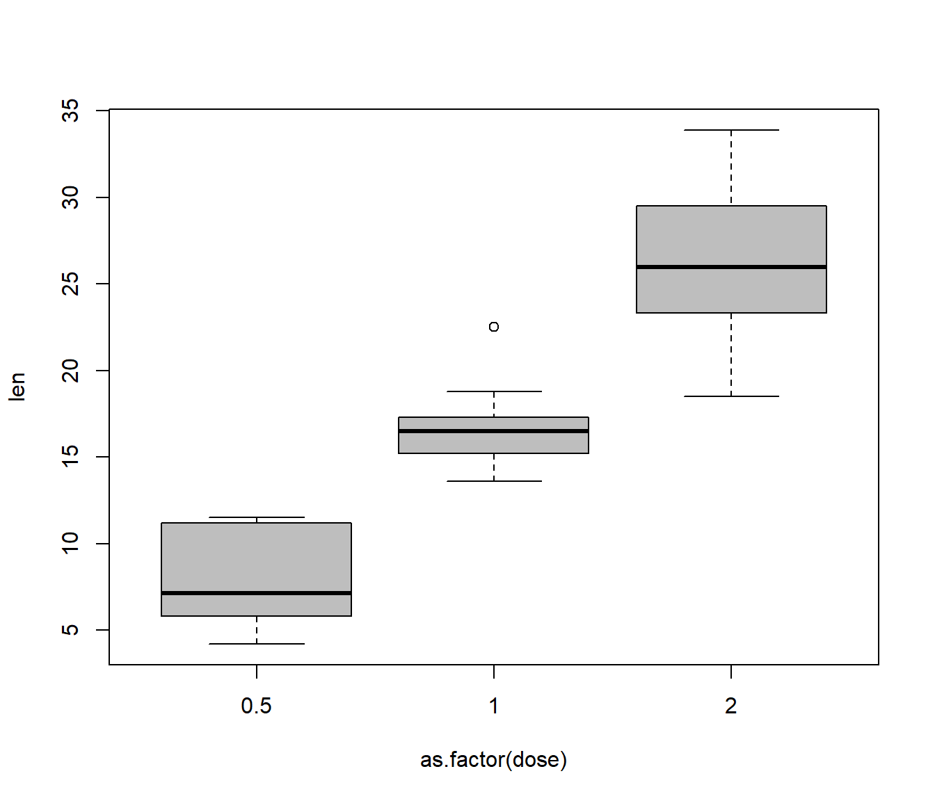
    Bartlett test of homogeneity of variances

data:  len by as.factor(dose)
Bartlett's K-squared = 4.5119, df = 2, p-value = 0.1048
21.1.2 Initial Comments
The as.factor() function tells R to regard the (numeric
variable) dose as a factor.
The levels are ordered in the natural way.
The box plot is slightly suggestive of a change of dispersion (spread) in the response between the groups, but Bartlett’s test does not provide clear evidence of heteroscedasticity (P-value is P=0.1048).
From the plot it seems highly plausible that mean tooth growth depends on vitamin C levels.
21.2 Nesting of Linear Effects
Consider a one factor experiment in which the factor levels are defined in terms of a numerical variable x. In other words, all individuals at factor level j take the same value of x for this variable (\(j=1,2,\ldots,K\)).
We could fit a simple linear regression model to the data:
\[M0: Y_i = \beta_0 + \beta_1 x_i + \varepsilon_i~~~~~~(i=1,2,\ldots,n)\]
We could also fit a standard one-way factorial model which can be written as a multiple regression model:
\[M1: Y_i = \mu + \alpha_2 z_{i2} + \cdots + \alpha_K z_{iK}+\varepsilon_i~~~~~~(i=1,2,\ldots,n)\]
where \(z_{ij}\) is the indicator variable for unit i being at factor level j as usual.
The difference between these models is that the simple regression model (\(M0\)) assumes that the expected values (means) of the response for each level of the factor follow a straight line. On the contrary, the one-way model (\(M1\)) allows the mean response to vary arbitrarily across the levels of the factor. Therefore, the \(M0\) model will be preferred if the relationship between the factor and the response is linear. The \(M1\) model will be preferred if their relationship is not linear.
We can show that model \(M0\) is nested within model \(M1\). It follows that we can compare models \(M0\) (the simpler one) and \(M1\) (the more complex one) using an F test.
Specifically, we will test H0: model \(M0\) adequate; versus H1: model \(M0\) not adequate, using the F test statistic:
\[F = \frac{[RSS_{M0} - RSS_{M1}]/(K-2)}{RSS_{M1}/(n-K)}.\]
\(M1\) has n-K residual degrees of freedom.
The difference in the number of parameters between the models is K-2.
Hence the F-statistic has K-2, n-K degrees of freedom.
If fobs is the observed value of the test statistic, and X is a random variable from an FK-2,n-K distribution, then the P-value is given by
\[P= P(X \ge f_{obs})\]
Retention of H0 indicates that a simple linear regression model is adequate; i.e. the effect of the variable x is adequately modelled as linear.
Rejection of H0 indicates that any association between y and x is non-linear.
21.3 Analysis of the Guinea Pig Tooth Data
R Code for Model \(M0\):
Call:
lm(formula = len ~ dose, data = TG)

Residuals:
    Min      1Q  Median      3Q     Max
-8.2264 -2.6029  0.0814  2.2288  7.4893

Coefficients:
            Estimate Std. Error t value Pr(>|t|)
(Intercept)    3.295      1.427   2.309   0.0285 *
dose          11.716      1.079  10.860 1.51e-11 ***
---
Signif. codes:  0 '***' 0.001 '**' 0.01 '*' 0.05 '.' 0.1 ' ' 1

Residual standard error: 3.685 on 28 degrees of freedom
Multiple R-squared:  0.8082,    Adjusted R-squared:  0.8013
F-statistic: 117.9 on 1 and 28 DF,  p-value: 1.509e-11
R Code for Model \(M1\):
Call:
lm(formula = len ~ as.factor(dose), data = TG)

Residuals:
   Min     1Q Median     3Q    Max
-7.640 -2.248 -0.455  2.027  7.760

Coefficients:
                 Estimate Std. Error t value Pr(>|t|)
(Intercept)         7.980      1.109   7.196 9.71e-08 ***
as.factor(dose)1    8.790      1.568   5.605 6.02e-06 ***
as.factor(dose)2   18.160      1.568  11.580 5.58e-12 ***
---
Signif. codes:  0 '***' 0.001 '**' 0.01 '*' 0.05 '.' 0.1 ' ' 1

Residual standard error: 3.507 on 27 degrees of freedom
Multiple R-squared:  0.8324,    Adjusted R-squared:   0.82
F-statistic: 67.07 on 2 and 27 DF,  p-value: 3.357e-11
R Code to compare the models:
Analysis of Variance Table

Model 1: len ~ dose
Model 2: len ~ as.factor(dose)
  Res.Df    RSS Df Sum of Sq      F  Pr(>F)
1     28 380.15
2     27 332.00  1    48.146 3.9155 0.05813 .
---
Signif. codes:  0 '***' 0.001 '**' 0.01 '*' 0.05 '.' 0.1 ' ' 1
21.3.1 Conclusions
The relationship between tooth length and vitamin C is found to be statistically significant using both the linear regression model (P<0.0001) and the factor model (P<0.0001).
The F test for comparing the linear effect and factor model gives an F-statistic of \(f=3.92\) on \(K - 2 = 1\) and \(n - K = 27\) degrees of freedom.
The corresponding P-value is \(P=0.058\). We would retain H0 at the 5% significance level, but there is certainly some evidence to doubt that the relationship should be modelled as a linear effect.
21.4 Example: North Shore Rents 2021
We consider the relationship between the asking rent and the number of bedrooms available, for accommodation advertised on Auckland’s North Shore, on 15 May 2021. (Source: Trademe). A few extremely high-priced outliers have been excluded. One-bedroom accommodation includes studio apartments. Is it reasonable to assume the relationship between rents and the number of bedrooms is linear?
## NSrent = read.csv(file = "NSrent2021.csv", header = TRUE)
boxplot(rent ~ as.factor(bedrooms), data = NSrent)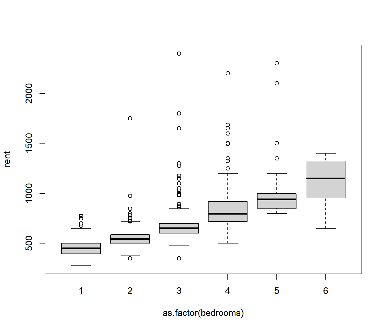
The boxplots indicate the medians rise fairly linearly with the number of bedrooms, so we might assume this is true for the means as well. There is a problem with heteroscedasticity, but we will set that aside for now.
Call:
lm(formula = rent ~ bedrooms, data = NSrent)

Residuals:
    Min      1Q  Median      3Q     Max
-482.00  -90.44  -38.88   30.49 1689.87

Coefficients:
            Estimate Std. Error t value Pr(>|t|)
(Intercept)  288.261     18.849   15.29   <2e-16 ***
bedrooms     140.623      6.178   22.76   <2e-16 ***
---
Signif. codes:  0 '***' 0.001 '**' 0.01 '*' 0.05 '.' 0.1 ' ' 1

Residual standard error: 191.3 on 709 degrees of freedom
Multiple R-squared:  0.4222,    Adjusted R-squared:  0.4214
F-statistic: 518.1 on 1 and 709 DF, p-value: < 2.2e-16Analysis of Variance Table
Model 1: rent ~ bedrooms
Model 2: rent ~ as.factor(bedrooms)
Res.Df RSS Df Sum of Sq F Pr(>F)
1 709 25933643
2 705 25697610 4 236033 1.6189 0.1676The first lm indicates that there is a significant linear relationship between rent and the number of bedrooms.
The anova comparison shows that we do not need to suppose the relationship is nonlinear: i.e. the linear trend is sufficient to describe the relationship (p-value of 0.1676). This is good, because a simple straight-line model is easy to interpret.
As for the heteroscedasticity, we might be tempted to try to stabilise the variance by a transforming the bedrooms variable, but that would destroy the simplicity of the linear relationship. Instead, in a later topic we will allow for the heteroscedasticity by using a method called weighted least squares.
21.5 Analysis of Genetic Data
A haplotype is a unit of genetic information contained on a single chromosome. Because chromosomes come in pairs (one inherited from each parent), an individual may have either zero, one or two copies of any given haplotype. The effects of a haplotype on some phenotype (measurable physical attribute) may or may not be linear in the number of copies of the haplotype.

A measure of cholesterol was recorded on 35 subjects. Of these, 8 have zero copies, 16 had one copy, and 11 had two copies of a particular haplotype.
Fitting the number of copies of the haplotype as a linear effect gave a residual sum of squares of \(153.2\).
Fitting the number of copies of the haplotype as a factor gave a residual sum of squares of \(126.2\).