Lecture 26 Comparison of general linear models
Loading required package: carData
Attaching package: 'car'The following object is masked from 'package:dplyr':
recodeThe following object is masked from 'package:purrr':
someWelcome to emmeans.
Caution: You lose important information if you filter this package's results.
See '? untidy'
Attaching package: 'kableExtra'The following object is masked from 'package:dplyr':
group_rows
Attaching package: 'scales'The following object is masked from 'package:purrr':
discardThe following object is masked from 'package:readr':
col_factor
Attaching package: 'gridExtra'The following object is masked from 'package:dplyr':
combine26.1 Learning objectives
By the end of this in-class session you will be able to:
Recall the five canonical GLM forms from Lecture 25 and how parameterization and contrasts affect interpretation.
Map natural orderings of GLMs and identify which pairs are nested.
Conduct partial F tests for nested GLMs and interpret RSS, df, F, and P.
Explain why p-values can change when multiple models are passed to
anova().Compare three Samara models and select a defensible specification.
Transfer the workflow to a second dataset on body fat with one covariate and one factor.
26.2 Quick recall of Lecture 25
Five canonical model forms for one factor A and one covariate x:
- Separate slopes:
Y ~ A + A:xor equivalentlyY ~ A * x - Parallel slopes:
Y ~ A + x - Single regression line:
Y ~ x - Intercepts only by level:
Y ~ A - Null model:
Y ~ 1
Equivalence of parameterizations: two formulas can span the same model space even if coefficients differ. Same fitted values implies same residuals and identical SSE.
Centering covariates: centering turns the intercept into the mean response at average x, which improves interpretability in interaction models.
26.3 Comparison on Nested Linear Models
For any linear model \(M0\) nested within \(M1\), we can test:
\(H_0\): \(M0\) adequate vs
\(H_1\): \(M0\) not adequate.
using an F test.
The hypotheses can be stated in terms of parameters of model \(M1\).
The F test statistic is
\[F = \frac{[RSS_{M0} - RSS_{M1}]/d}{RSS_{M1}/r}\] where d is the difference in the number of (regression) parameters between the models, and r is the residual degrees of freedom for \(M1\).
If \(H_0\) is correct then F has an F distribution with \(d,r\) degrees of freedom.
Extreme large values of the test statistic provide evidence against \(H_0\).
Hence if \(f_{obs}\) is the observed value of the test statistic, and X is a random variable from an \(F_{d,r}\) distribution, then the P-value is given by \(P= P(X \ge f_{obs})\)
This test can be carried out in R using anova(M0, M1) where M0 and M1 are respectively the \(M0\) and \(M1\) fitted models.
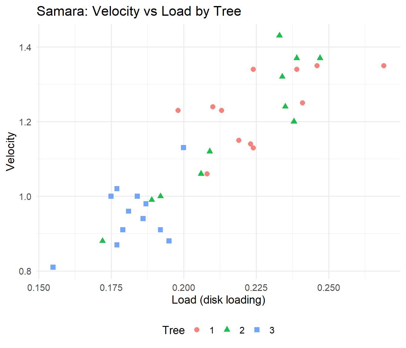
26.4 The Samara Data revisited
Recall that we were modelling the mean speed of fall of samara (fruit from a maple tree) as a function of the disk loading (a covariate) and the tree from which it fell (a factor) for each fruit.
We fitted separate linear regressions for each of the three trees.
We shall now consider simpler models:
- Parallel regressions for each tree (i.e. equal slope for
Loadfor all trees); - A single regression model for every fruit (i.e. equal slope and intercept for each tree).
We shall compare these models with each other, and with the separate regressions model.
Grab the data here: samara.csv
26.5 Natural ordering of GLMs and nesting
We focus on the nesting relations for one factor Tree and covariate Load:
- Null ⊂ Intercepts-only ⊂ Parallel slopes ⊂ Separate slopes
Single line vs Intercepts-only are not nested when groups differ in mean at x = 0.
Valid partial F tests require true nesting and common error variance.
We fit:
- M2: Separate regressions:
Velocity ~ Tree + Load + Tree:Load - M1: Parallel regressions:
Velocity ~ Tree + Load - M0: Single regression:
Velocity ~ Load
M2_sep <- lm(Velocity ~ Tree + Load + Tree:Load, data = Samara)  # separate slopes
M1_par <- lm(Velocity ~ Tree + Load, data = Samara)  # parallel slopes
M0_one <- lm(Velocity ~ Load, data = Samara)  # single line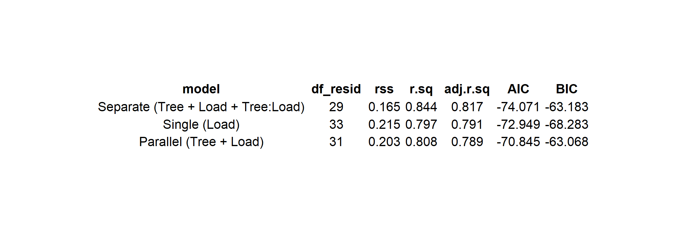
Figure 26.1: Model summaries with RSS, df, R^2, AIC, BIC
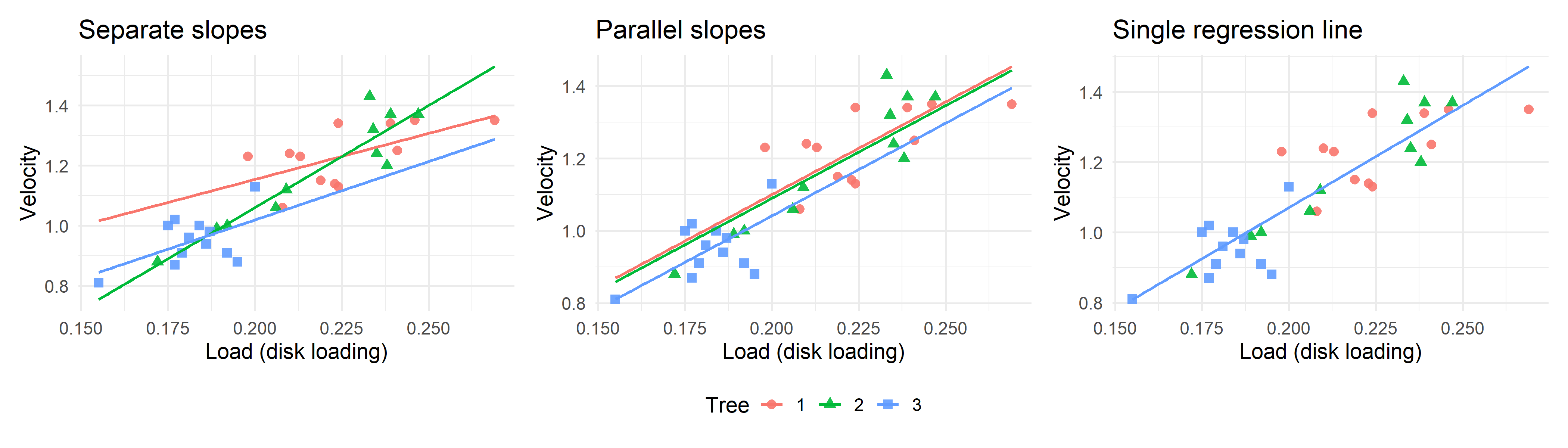
26.6 Visualizing fitted lines
Let’s look at these fits visually to remind ourselves what the data looks like and how the models differ.
26.7 Pairwise nested comparisons with partial F tests
Analysis of Variance Table

Model 1: Velocity ~ Tree + Load
Model 2: Velocity ~ Tree + Load + Tree:Load
  Res.Df     RSS Df Sum of Sq     F  Pr(>F)
1     31 0.20344
2     29 0.16549  2  0.037949 3.325 0.05011 .
---
Signif. codes:  0 '***' 0.001 '**' 0.01 '*' 0.05 '.' 0.1 ' ' 1
26.8 Pairwise nested comparisons with partial F tests continued
Analysis of Variance Table

Model 1: Velocity ~ Load
Model 2: Velocity ~ Tree + Load
  Res.Df     RSS Df Sum of Sq      F Pr(>F)
1     33 0.21476
2     31 0.20344  2  0.011322 0.8626 0.4319
26.9 Pairwise nested comparisons with partial F tests continued
Analysis of Variance Table

Model 1: Velocity ~ Load
Model 2: Velocity ~ Tree + Load + Tree:Load
  Res.Df     RSS Df Sum of Sq      F  Pr(>F)
1     33 0.21476
2     29 0.16549  4  0.049272 2.1585 0.09885 .
---
Signif. codes:  0 '***' 0.001 '**' 0.01 '*' 0.05 '.' 0.1 ' ' 1
26.10 All models in one call and denominator effect
Analysis of Variance Table

Model 1: Velocity ~ Load
Model 2: Velocity ~ Tree + Load
Model 3: Velocity ~ Tree + Load + Tree:Load
  Res.Df     RSS Df Sum of Sq     F  Pr(>F)
1     33 0.21476
2     31 0.20344  2  0.011322 0.992 0.38306
3     29 0.16549  2  0.037949 3.325 0.05011 .
---
Signif. codes:  0 '***' 0.001 '**' 0.01 '*' 0.05 '.' 0.1 ' ' 1
Note: The p-value for M0 vs M1 can change because the denominator uses the largest model in the call. Decide a maximal model ahead of time or clearly document the sequential plan.
26.11 Manual check of the F test
We verify M1 vs M2 by hand.
Remember \[ F = \frac{(RSS_{M1} - RSS_{M2})/d}{RSS_{M2}/r} \]
rss_M1 <- sum(residuals(M1_par)^2)
rss_M2 <- sum(residuals(M2_sep)^2)
d <- attr(logLik(M2_sep), "df") - attr(logLik(M1_par), "df")  # number of added parameters
r <- df.residual(M2_sep)  # residual df in larger model
Fval <- ((rss_M1 - rss_M2)/d)/(rss_M2/r)
pval <- pf(Fval, d, r, lower.tail = FALSE)| comparison | d | r | F | Pr(>F) |
|---|---|---|---|---|
| M1 vs M2 | 2 | 29 | 3.325032 | 0.050107 |
26.12 Diagnostics checklist for the chosen model
chosen <- M1_par
p1 <- ggplot(data.frame(fitted = fitted(chosen), resid = resid(chosen)), aes(fitted,
    resid)) + geom_point() + geom_hline(yintercept = 0, linetype = 2) + labs(title = "Residuals vs Fitted") +
    theme_minimal(base_size = 13)
p2 <- ggplot(data.frame(stdres = rstandard(chosen)), aes(sample = stdres)) + stat_qq() +
    stat_qq_line() + labs(title = "Normal Q-Q") + theme_minimal(base_size = 13)
p1 | p2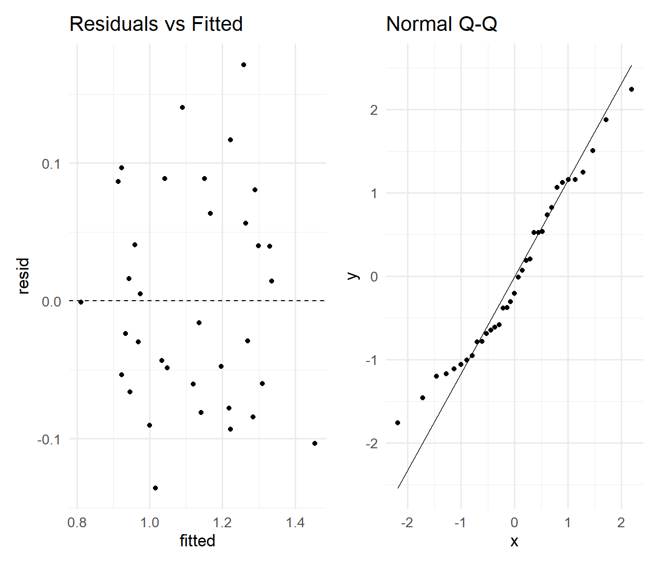
26.13 Body Fat case study
In this section, we are concerned with modelling a small data set on human body fat.
The response is percentage fat. Age is a numerical covariate, gender is a factor.
Grab the data here: fat.csv
Various model comparisons and model summaries are provided. Decide which is the best model, and write down the fitted model equation for males and females.
Columns: Percent.Fat response, Age numeric, Gender factor.
p_fat <- ggplot(Fat, aes(x = Age, y = Percent.Fat, color = Gender, shape = Gender)) +
    geom_point(size = 2.6, alpha = 0.9) + labs(title = "Percent Body Fat vs Age by Gender",
    x = "Age", y = "Percent Fat") + theme_minimal(base_size = 14) + theme(legend.position = "bottom")
p_fat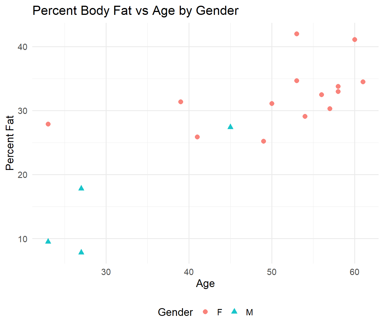
26.14 Three models and comparisons
F0 <- lm(Percent.Fat ~ Age, data = Fat)
F1 <- lm(Percent.Fat ~ Gender + Age, data = Fat)
F2 <- lm(Percent.Fat ~ Gender + Age + Gender:Age, data = Fat)

anova(F0, F1)
Analysis of Variance Table
Model 1: Percent.Fat ~ Age
Model 2: Percent.Fat ~ Gender + Age
Res.Df RSS Df Sum of Sq F Pr(>F)
1 16 529.66
2 15 360.88 1 168.79 7.0157 0.01824 *
---
Signif. codes: 0 '***' 0.001 '**' 0.01 '*' 0.05 '.' 0.1 ' ' 1Analysis of Variance Table
Model 1: Percent.Fat ~ Gender + Age
Model 2: Percent.Fat ~ Gender + Age + Gender:Age
Res.Df RSS Df Sum of Sq F Pr(>F)
1 15 360.88
2 14 282.02 1 78.853 3.9144 0.0679 .
---
Signif. codes: 0 '***' 0.001 '**' 0.01 '*' 0.05 '.' 0.1 ' ' 1Since we are talking about a one degree of freedom difference, the p-value from anova(F1, F2) is the same as the p-value for the interaction term in F2, namely 0.0679. So we don’t use the interaction model.
Similarly the difference between the first two models is one df, so the p-value from anova(F0, F1) would be the same as for the coefficient of GenderM, namely 0.0182.
So we need to use the second model.
26.15 Selected model terms
Call:
lm(formula = Percent.Fat ~ Gender + Age, data = Fat)

Residuals:
   Min     1Q Median     3Q    Max
-6.638 -3.455 -1.103  3.297  8.952

Coefficients:
            Estimate Std. Error t value Pr(>|t|)
(Intercept)  15.0708     6.2243   2.421   0.0286 *
GenderM      -9.7914     3.6966  -2.649   0.0182 *
Age           0.3392     0.1196   2.835   0.0125 *
---
Signif. codes:  0 '***' 0.001 '**' 0.01 '*' 0.05 '.' 0.1 ' ' 1

Residual standard error: 4.905 on 15 degrees of freedom
Multiple R-squared:  0.7461,    Adjusted R-squared:  0.7123
F-statistic: 22.04 on 2 and 15 DF,  p-value: 3.424e-05
26.16 Fitted equations for the selected model
If we select the parallel slopes F1 with treatment contrasts and Gender coded with F as reference:
Females:
E[Fat] = β0 + β_Age * AgeMales:
E[Fat] = (β0 + β_GenderM) + β_Age * Age
co <- coef(F1)
beta0 <- unname(co["(Intercept)"])
beta_age <- unname(co["Age"])
beta_male <- unname(co["GenderM"])
tibble(model = c("Females", "Males"), equation = c(sprintf("Fat = %.2f + %.2f * Age",
    beta0, beta_age), sprintf("Fat = %.2f + %.2f * Age", beta0 + beta_male, beta_age))) |>
    kable(caption = "Fitted equations by Gender (parallel slopes model)") |>
kable_styling(full_width = FALSE)| model | equation |
|---|---|
| Females | Fat = 15.07 + 0.34 * Age |
| Males | Fat = 5.28 + 0.34 * Age |
26.17 Reporting template
- State the model forms, nesting, and the scientific contrast.
- Report RSS, df, F, and p with the denominator model identified.
- Add a sentence on diagnostics and effect interpretation.
- If two models are close, prefer the simpler one for clarity unless the complex model adds needed scientific nuance.