Lecture 15 Models with binary predictors
Let’s go back to the Climate data example, which had two binary predictors NorthIsland and Sea. In this lecture we will focus on the predictor NorthIsland only.
We can briefly examine the effects of this predictor via a boxplot. NorthIsland seems to have an effect on temperature, but is the effect statistically significant?
N.B. Download Climate.csv to replicate the following examples.
## Climate <- read.csv(file = "Climate.csv", header = TRUE, row.names = 1)
boxplot(MnJlyTemp ~ NorthIsland, data = Climate)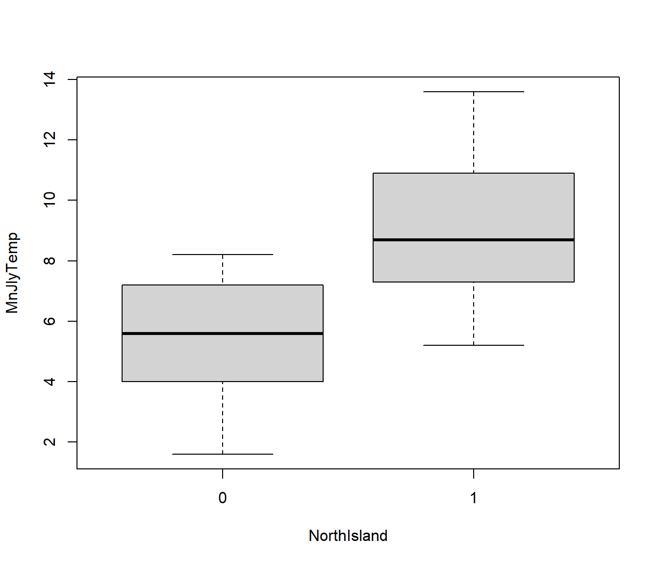
15.1 Idea of comparing groups using lm()
Suppose we denote the \(i\)th data value (response) from group \(j\) by \(Y_{ij}\), where \(j= 0,1\) and \(i=1,2,…,n_0\) or \(1,2,…,n_1\) respectively. Thus the group means are \(\mu_0\) and \(\mu_1\) .
One way to analyse the data would be to use a two-sample t-test to test the hypothesis \(H_0:~~\mu_0= \mu_1\) versus \(H_1:~~\mu_0 \ne\mu_1\). You may have been introduced to such tests in your first-year statistics course.
Another way of writing down the hypothesis (which will turn out to be convenient) is to treat one group as a “baseline group” with mean \(\mu\) and the other group as a shifted or “treatment” group with mean \(\mu+\delta\). Then the hypotheses become \(H_0:~\delta=0\) vs versus \(H_1:~\delta\ne 0\).
There is a definite advantage in writing the hypothesis this way. Namely, we can easily put the test into the linear model framework, since the regression models are written in the form where we are testing whether a slope (which will be \(\delta\)) equals zero.
To write it this way, define an indicator variable as \(z_i = 0\) if the datum is in group 0, and \(z_i=1\) if if is in group 1.
Then we can write a formula for the response as
\[ E[Y_i] = \mu + \delta z_i = \beta_0 + \beta_1 z_i\]
where \(\beta_0 = \mu\) and \(\beta_1 = \delta\).
In other words the two-group comparison can be put in the same form as a linear regression. So all we would need to do is:
set up the group indicator variable z,
regress Y on z and
test the hypothesis that the slope =0.
15.2 Testing using lm()
If we want to test the significance of the relationship between NorthIsland and temperature, we can use lm(). Remember lm() assumes the variance of residuals does not depend on the values of the predictor. From the boxplot it looks like this assumption is justified.
Call:
lm(formula = MnJlyTemp ~ NorthIsland, data = Climate)

Residuals:
    Min      1Q  Median      3Q     Max
-3.8647 -1.7421 -0.1034  1.8079  4.5579

Coefficients:
            Estimate Std. Error t value Pr(>|t|)
(Intercept)   5.4647     0.5187  10.536 3.02e-12 ***
NorthIsland   3.5774     0.7140   5.011 1.66e-05 ***
---
Signif. codes:  0 '***' 0.001 '**' 0.01 '*' 0.05 '.' 0.1 ' ' 1

Residual standard error: 2.139 on 34 degrees of freedom
Multiple R-squared:  0.4248,    Adjusted R-squared:  0.4078
F-statistic: 25.11 on 1 and 34 DF,  p-value: 1.665e-05
The t-test for the slope of the model is significant (p-value = 1.66e-05), indicating that there is a significant difference between the mean of the two groups.
15.3 Testing using t.test()
Since this is a simple two-group comparison, we can also investigate using a standard two-sample t.test, which gives basically the same conclusion.
    Welch Two Sample t-test

data:  MnJlyTemp by NorthIsland
t = -5.0114, df = 33.581, p-value = 1.711e-05
alternative hypothesis: true difference in means between group 0 and group 1 is not equal to 0
95 percent confidence interval:
 -5.028803 -2.125996
sample estimates:
mean in group 0 mean in group 1
       5.464706        9.042105
On close inspection you will see that the p-value and df are not exactly the same as for the lm().
The reason is that the default settings for t.test() do not assume equal variances, and so uses a method called Welch’s method. Essentially it does a fudge on the df to make the t-distribution work.
If we want to get exactly the same results in the t.test() as in the lm(), then we need to set the var.equal=TRUE option.
    Two Sample t-test

data:  MnJlyTemp by NorthIsland
t = -5.0105, df = 34, p-value = 1.665e-05
alternative hypothesis: true difference in means between group 0 and group 1 is not equal to 0
95 percent confidence interval:
 -5.028371 -2.126428
sample estimates:
mean in group 0 mean in group 1
       5.464706        9.042105
In this case the t statistics, df and p-value are equal to those from lm.
15.4 How do we know whether to assume equal variances?
A simple rule of thumb we can use is that if the standard deviation of residuals for the two groups does not differ by more than a factor of 2, then we can assume equal variances.
[1] 0.9971634(Note that the with() function allows us to use the variables from the Climate dataframe without writing Climate$; MnJlyTemp[NorthIsland == 0] gives us the temperatures for observations not in the North Island). Clearly the ratio is much less than 2.
Preferably, we will perform a formal statistical test of \(H_0: \sigma_0^2 = \sigma_1^2\) (i.e. variances are equal) vs \(H_1:\) variances are not equal.
There are two tests commonly used: Bartlett’s test (which depends more on the errors being normally distributed) and Levene’s test (which works even if the data are not normal).
We will normally use the Levene’s test. The corresponding R function is available through the car package.
    Bartlett test of homogeneity of variances

data:  MnJlyTemp by factor(NorthIsland)
Bartlett's K-squared = 0.00013276, df = 1, p-value = 0.9908Levene's Test for Homogeneity of Variance (center = median)
Df F value Pr(>F)
group 1 2e-04 0.9902
34 Note the use of the factor() function to indicate that we want to treat the NorthIsland variable as a group indicator variable (rather than a numerical variable).
The p-value for both these tests is large, which confirms that, for the Climate data, we have no reason to doubt the equal variance assumption.
15.5 Models for a single numeric predictor and a binary group variable
Binary predictors can also be used to deal with changes in slope between two groups.
For example, in their book “Regression Analysis by Example”, Chatterjee and Price present some data on the impact of amount of revision impacts scores in an English exam differently for boys and girls. Let:
- \(Y_i\) = score in English exam,
- \(x_i\) = number of hours spent in revision,
- \(z_i\) = sex (0 for boys, 1 for girls).
N.B. Download EnglishExam.csv if you want to replicate the following examples.
  resulty revision sex
1      64       12   1
2      43       14   1
3      37        4   0
4      50        5   0
5      52        6   0
6      23        6   1
Looking at the data graphically we see:
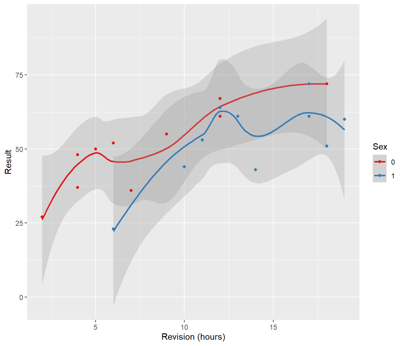
The question we are asking is: should the lines for boys and girls have a different slope?
To answer this question, we need to fit a model in which boys and girls have different slopes. As in the previous section, it is convenient to test for a difference in slope by setting a baseline group (say, the boys) with slope \(\beta_1\), and expressing the slope for the girls group as a shifted slope \(\beta_1 + \delta\). That is, we want a model with the following response:
\[E[Y_i] = \beta_0 + \beta_1 x_i ~\mbox{ for boys, and}\] \[E[Y_i] = \beta_0 + (\beta_1 + \delta) x_i ~\mbox{ for girls}\]
The group indicator variable \(z_i\) is very convenient to construct the appropriate model:
\[E[Y_i] = \beta_0 + (\beta_1 + \delta z_i) x_i = \beta_0 + \beta_1 x_i + \delta x_i z_i\]
Here, \(x_i z_i\) corresponds to a new variable that is equal to 0 for boys and to \(x_i\) for girls. In order to fit the model with lm() in the usual way, we can easily construct this new variable:
  resulty revision sex revisionGirls
1      64       12   1            12
2      43       14   1            14
3      37        4   0             0
4      50        5   0             0
5      52        6   0             0
6      23        6   1             6
We can now fit the model:
English.lm1 <- lm(resulty ~ revision, data = English)
English.lm2 <- lm(resulty ~ revision + revisionGirls, data = English)

summary(English.lm2)
Call:
lm(formula = resulty ~ revision + revisionGirls, data = English)

Residuals:
     Min       1Q   Median       3Q      Max
-16.4760  -5.8961   0.4898   7.4113  13.4149

Coefficients:
              Estimate Std. Error t value Pr(>|t|)
(Intercept)    28.3669     4.9866   5.689 2.67e-05 ***
revision        2.7342     0.5644   4.844 0.000152 ***
revisionGirls  -0.8827     0.3954  -2.232 0.039334 *
---
Signif. codes:  0 '***' 0.001 '**' 0.01 '*' 0.05 '.' 0.1 ' ' 1

Residual standard error: 9.074 on 17 degrees of freedom
Multiple R-squared:  0.6111,    Adjusted R-squared:  0.5653
F-statistic: 13.35 on 2 and 17 DF, p-value: 0.0003266Analysis of Variance Table
Model 1: resulty ~ revision
Model 2: resulty ~ revision + revisionGirls
Res.Df RSS Df Sum of Sq F Pr(>F)
1 18 1809.9
2 17 1399.7 1 410.29 4.9833 0.03933 *
---
Signif. codes: 0 '***' 0.001 '**' 0.01 '*' 0.05 '.' 0.1 ' ' 1The coefficient associated with our constructed variable revisionGirls is significant (p-value \(\approx 0.04\)), which indicates that there is a difference in the slope between boys and girls.