Lecture 4 Linear Regression Modelling with R
In this lecture we will look at simple linear regression modelling in R.
We shall use R to fit models (i.e. estimate the unknown parameters in models).
We shall discuss the interpretation of output from R.
4.1 The lm() Command
R uses the linear model command to fit models of this type.
The basic syntax is lm(formula, data) where:
formulais the model formula (required argument)datais the data frame in use (optional).- Variables are taken from your stored objects if no data frame is specified.
4.2 Analysis of the Pulse Data:
## PulseData <- read.csv(file = "https://r-resources.massey.ac.nz/data/161251/pulse.csv",
##     header = TRUE)
summary(PulseData)
Height Pulse
Min. :145.0 Min. : 64.0
1st Qu.:162.2 1st Qu.: 80.0
Median :169.0 Median : 80.0
Mean :168.7 Mean : 82.3
3rd Qu.:175.0 3rd Qu.: 84.0
Max. :185.0 Max. :116.0 It is common to use names for your models that make sense, especially to the person you will work with the most in future (you, yourself!). Remember, your future self will be pretty annoyed that your current self isn’t going to be able to answer questions about your funny selections of names, so go easy on yourself by being clear with your work.
The most common convention is to use a name that shows what data was used and what type of model was created. We will see <data>.lm lots in this course!
Call:
lm(formula = Pulse ~ 1 + Height, data = PulseData)

Residuals:
    Min      1Q  Median      3Q     Max
-16.666  -4.876  -1.520   3.424  33.012

Coefficients:
            Estimate Std. Error t value Pr(>|t|)
(Intercept)  46.9069    22.8793   2.050   0.0458 *
Height        0.2098     0.1354   1.549   0.1279
---
Signif. codes:  0 '***' 0.001 '**' 0.01 '*' 0.05 '.' 0.1 ' ' 1

Residual standard error: 8.811 on 48 degrees of freedom
Multiple R-squared:  0.04762,   Adjusted R-squared:  0.02778
F-statistic:   2.4 on 1 and 48 DF,  p-value: 0.1279
The most commonly sought numbers in that output are the coefficients
(Intercept)      Height
  46.906927    0.209774
But in simple regression, we often want to see how these coefficients create a line, and how that line looks alongside our data. We can do this in a simple plot() or a fancy ggplot(). N.B. Other visualisations also exist! Make an active choice.
plot(Pulse ~ Height, data = PulseData, ylab = "Resting pulse rate (beats per minute)",
    xlab = "Height (in centimeters) ")
abline(Pulse.lm)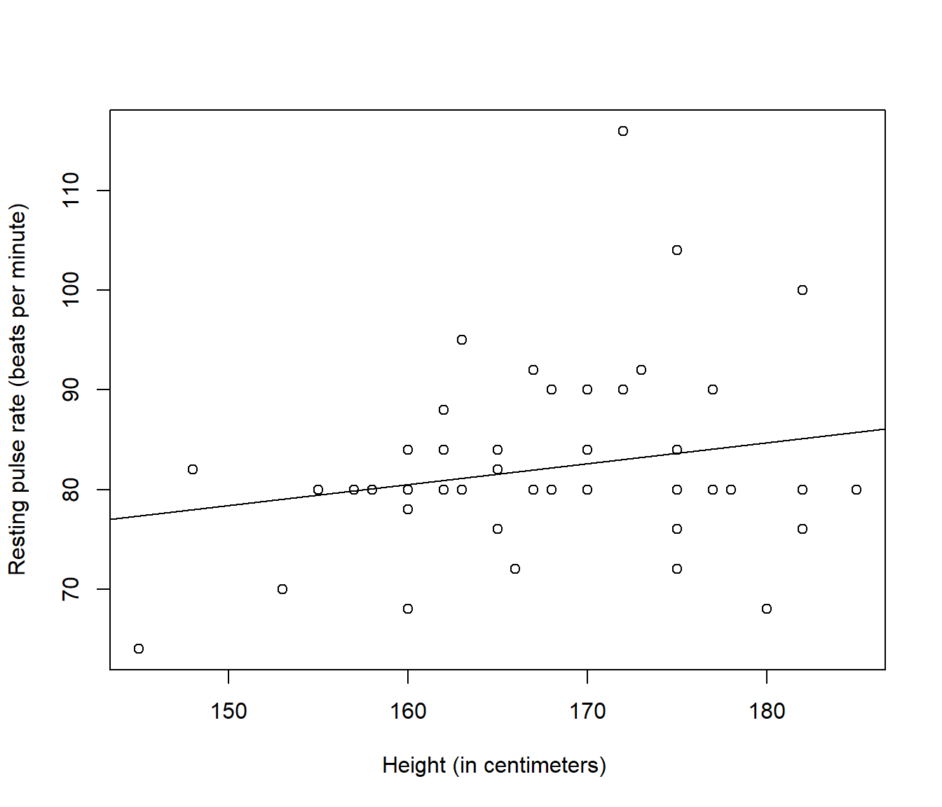
Figure 4.1: Plot of resting pulse rate (beats per minute) versus height (in centimeters) with fitted line added, for a sample of 50 hospital patients. Source: A Handbook of Small Data Sets by Hand, Daly, Lunn, McConway and Ostrowski.
library(ggplot2)
PulseData |>
    ggplot(mapping = aes(x = Height, y = Pulse)) + geom_point() + geom_smooth(method = "lm",
    se = FALSE) + ylab("Resting pulse rate (beats per minute)") + xlab("Height (in centimeters) ")
`geom_smooth()` using formula = 'y ~ x'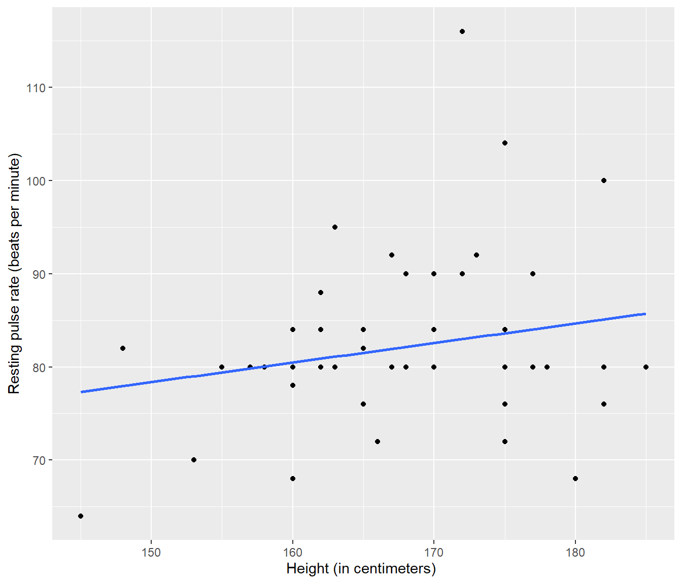
Figure 4.2: Plot of resting pulse rate (beats per minute) versus height (in centimeters) with fitted line added, for a sample of 50 hospital patients. Source: A Handbook of Small Data Sets by Hand, Daly, Lunn, McConway and Ostrowski.
4.2.2 Interpretation of Model for Pulse Data
The summary table of coefficients contains much relevant
information. We can get this part of the summary using the tidy() command.
| term | estimate | std.error | statistic | p.value |
|---|---|---|---|---|
| (Intercept) | 46.906927 | 22.8793281 | 2.050188 | 0.0458292 |
| Height | 0.209774 | 0.1354041 | 1.549245 | 0.1278917 |
The kable() command here makes the pretty table for presentation; you wouldn’t use it in an interactive situation.
The fitted model (i.e. model with parameters replaced by estimates) is \[E[\mbox{Pulse}] = 46.91 + 0.21 ~\mbox{Height}\]
4.2.3 Residual standard error
The error standard deviation, \(\sigma\), is estimated by s=8.811 (the residual standard error) according to the output.
The s is a very useful statistic, and highly interpretable. This is because about 95% of residuals will be within about (formula explained later) \(\pm t_{(n-2)}(0.025) ~~s \approx \pm 2~s\).
This converts to meaning that about 95% of data values \(y_i\) will be within \(2~ s\) above or below the line.
In the present case \(s\approx 8.8\) so most pulses will be within about \(\pm 17.6\) beats above or below the predicted value on the line. This simple mental calculation gives us an idea how accurate and useful our regression is likely to be for prediction (So, in fact, not very accurate or useful at all, in this example!)
It also means we can do a simple graph to help us find y values that are unusual (We will refine this graph later)
`geom_smooth()` using formula = 'y ~ x'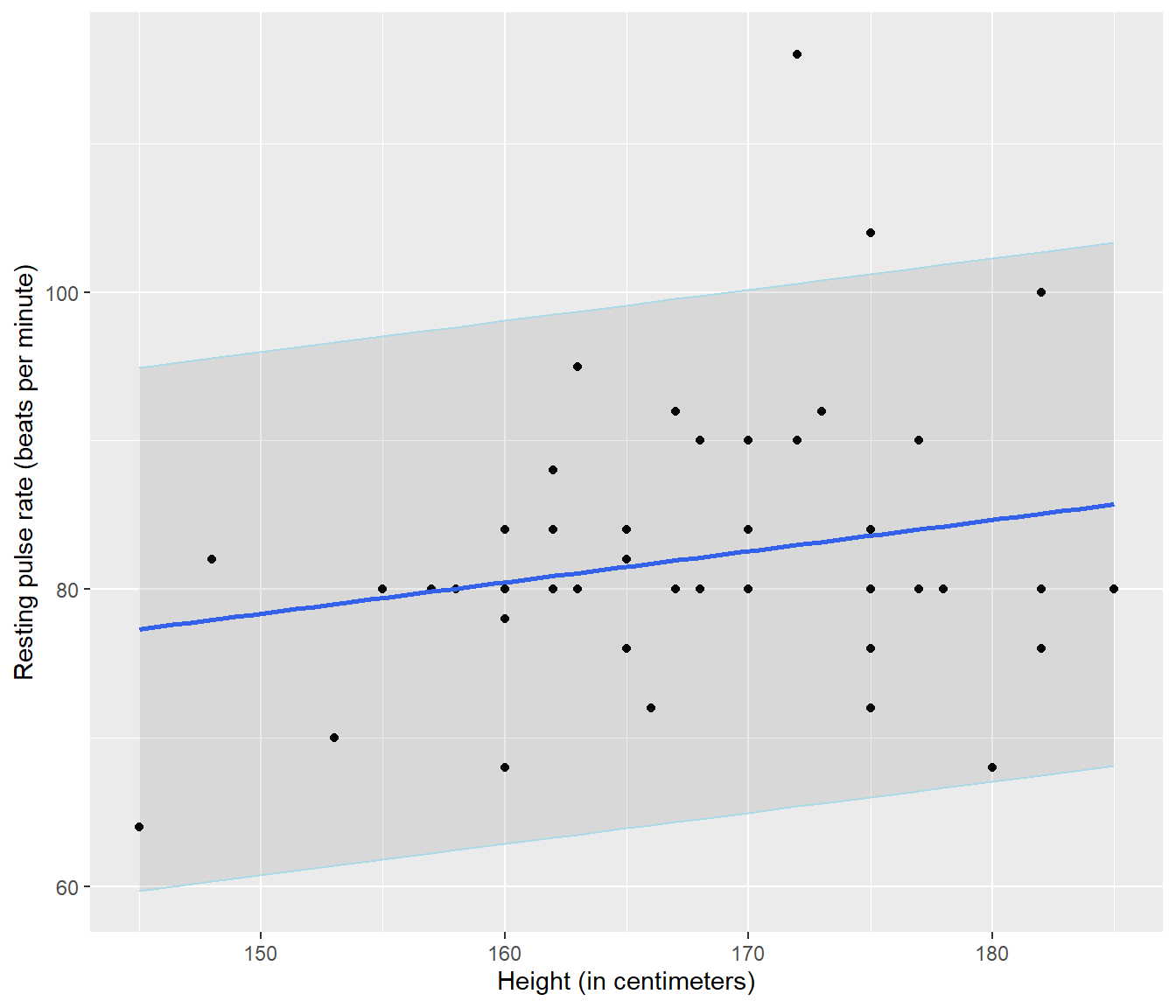
Figure 4.3: A fitted line added to a scatterplot of resting pulse rate against height. The grey area shows a plausible region within which 95% of observations should lie.
The graph illustrates that the model is really pretty poor, and also that there are two individuals whose pulse is much higher than is typical.
4.2.4 R2 for the Pulse Data
The (multiple) R-squared statistic, R2, is the square of the correlation between the observed and fitted responses.
It also has another name, the coefficient of determination.
It can be interpreted as the proportion of variation in the response that is explained by the predictor in the model. (In other words, how much the y values are determined (fixed) by the regression model)
Hence Height explains just R2 = 4.8% of the variation in the response according to the fitted model.
4.2.4.1 R hint:
You can find what different parts of the output are called, by applying the names() function to the summary() of a linear model you’ve fitted.
 [1] "call"          "terms"         "residuals"     "coefficients"
 [5] "aliased"       "sigma"         "df"            "r.squared"
[9] "adj.r.squared" "fstatistic" "cov.unscaled" [1] 0.04762205[1] 8.810716These “names” don’t change from model to model.
4.2.5 The estimated slope
The slope estimate, \(\hat{\beta_1} = 0.209774\) has associated standard error \(SE(\hat \beta_1) = 0.1354041.\)
For testing H0: \(\beta_1 = 0\) versus H1: \(\beta_1 \ne 0\), the t-test statistic is
\[t = \hat \beta_1 / SE(\hat \beta_1) = 0.210/0.135 = 1.5492447\]
The corresponding P-value is P=0.1278917, just like when we did the analysis by hand.
We conclude that the data provide no evidence of a (linear) relationship between resting pulse rate and height.
A nice presentation of this can be obtained using:
| term | estimate | std.error | statistic | p.value |
|---|---|---|---|---|
| (Intercept) | 46.906927 | 22.8793281 | 2.050188 | 0.0458292 |
| Height | 0.209774 | 0.1354041 | 1.549245 | 0.1278917 |
4.3 Confidence intervals for parameters
Generating the confidence interval for the parameters of our regression model is pretty simple and is achieved using the confint() command.
                  2.5 %     97.5 %
(Intercept)  0.90495433 92.9088990
Height      -0.06247409  0.4820221
This basic implementation of the confint() command has found 95% confidence intervals for both the slope and intercept parameters.
In this context, the interval for \(\beta_0\) is irrelevant, because there is no point trying to find a CI for y = Pulse when a person’s x = Height is zero.
Asking for only the slope’s interval, and adjusting the level of confidence are fairly easily achieved.
Even so, the interval for the slope parameter includes zero. Many people prefer to use confidence intervals over hypothesis tests, especially when communicating their findings.
4.4 Final Comments on the Model for Pulse Data
Our conclusion does not provide evidence that pulse is not related to height - that’s not the way hypothesis testing works.
Our conclusions are based on the assumption that the model is appropriate.
Failure of the model assumptions A1-A4 (described previously) would indicate an inappropriate model.
We need diagnostic tools to assess model adequacy.
4.5 Practical Exercises
We’ve now covered the basics needed to start the practical exercises which will be discussed in Week 2. You might take a look at the first one now.
4.2.1 Comments on the R code for the Pulse Data
The
read.csv()command reads (multivariate) data from a text file with commas separating the values.The option
header=TRUEindicates that the first line of the text file contains column headings (not data points).The
summary()command will typically give sensible output when applied to a variety of types of object. We saw it used to summarise the raw data, and to summarise the simple regression model we fitted.The formula
Pulse ~ 1 + Heightspecifies thatPulseis the response andHeightthe explanatory variable in the model. The1explicitly indicates inclusion of an intercept. (Most people leave it out.)The
geom_smooth()command adds a line fitted using the specifiedmethodfor fitting the model. Note that we used"lm"here so that this line matches the results from fitting a model usinglm()to this data.