Lecture 7 What to do When Assumptions Fail
In the previous lecture we looked at:
- the assumptions underlying the (simple) linear regression model;
- tools for detecting failure of the assumptions.
In this lecture we shall consider what to do if the model assumptions fail.
7.1 What to Do When You Find Outliers
A Reminder
- The existence of outliers impacts on all model assumptions.
- If there are outliers, check whether data have been mis-recorded (go back to data source if possible).
- If an outlier is not due to transcription errors, then it may need removing before refitting the model.
- In general one should refit model after removing a single outlier, because removal of one outlier can alter the fitted models and hence make other points appear less (or more) inconsistent with the model.
7.2 What to do When Assumption A1 Fails
Failure of A1 indicates that the relationship between the mean response and the predictor is not linear (as specified by the simple linear regression model).
Failure of this assumption is very serious — all conclusions from the model will be questionable.
One possible remedy is to transform the data. e.g. if responses curve upwards then a log transformation of responses may help.
However, important to recognize that any transformation of the response distribution will also effect the error variance. Hence fixing one problem (lack of linearity) by transformation may create another problem (heteroscedasticity).
An alternative approach is to use polynomial regression (covered later in the course).
7.3 What to do When Assumption A2 Fails
Failure of A2 occurs most frequently because the data exhibit serial correlation in time (or space).
Failure of this assumption will leave parameter estimates unbiased, but standard errors will be incorrect.
Hence failure of A2 will render test results and confidence intervals unreliable.
We will look at regression models for time series later in the course.
7.4 What to do When Assumption A3 Fails
Failure of this assumption will leave parameter estimates unbiased, but standard errors will be incorrect.
Hence failure of A3 will render test results and confidence intervals unreliable.
Perhaps most common form of heteroscedasticity is when error variance increases with the mean response.
A common strategy is to transform the response variable. (We will see this in an example later in this lecture.)
If the relationship looks linear, then a logarithmic transformation of both response and predictor variables can sometimes help in this case.
An alternative strategy is to use weighted linear regression (covered later in the course).
7.5 What to do When Assumption A4 Fails
Failure of the assumption of normality for the distribution of the errors is not usually a serious problem.
Removal of (obvious) outliers will typically improve the normality of the standardized residuals.
7.6 Using Transformations to correct for heteroscedasticity
N.B. this is a strategy not a recipe. There is a chance that a transformation can resolve the problem, but you will not find out if it was successful until it has been tried and evaluated.
7.7 Example: Fatalities on Mt Everest
Climbing Mt Everest is a dangerous activity. This dataset gives the number of fatalities among climbers, per year, from 1960-2019. Records date right back to 1922, but our focus is on the most recent and relevant years. The mountain was closed to climbers in 2020, while in 2021 there were fewer climbers allowed on the mountain than in previous years. Once we know that the number of climbers is as free to change as in the years before 2020, we must either restrict our analysis (Plan A), or find some way to incorporate that extra knowledge (Plan B). Plan B is too advanced for the purposes of today’s lecture so let’s stick with Plan A.
You could quite easily find plenty of articles online about this scenario. e.g. https://journals.plos.org/plosone/article?id=10.1371/journal.pone.0236919
Download Everest.csv if you want to replicate the examples below.
  Year Fatalities
1 1960          2
2 1961          0
3 1962          1
4 1963          1
5 1964          0
6 1965 0 Year Fatalities
55 2014 17
56 2015 19
57 2016 7
58 2017 5
59 2018 5
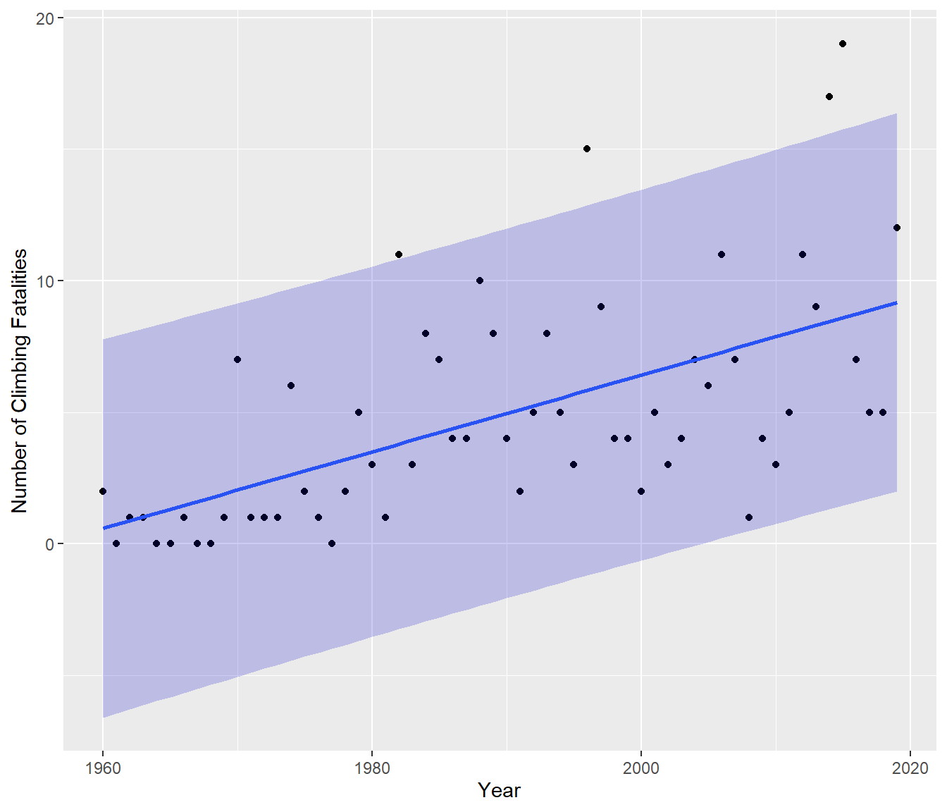
60 2019 12Taking a look at this data graphically:
`geom_smooth()` using formula = 'y ~ x'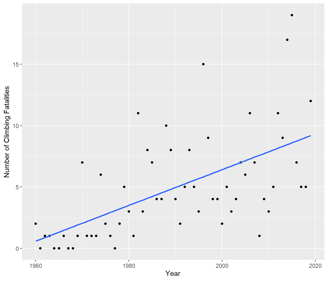
Clearly on average the number of Fatalities has been increasing. Fitting a simple model to this data and checking the assumptions gives…
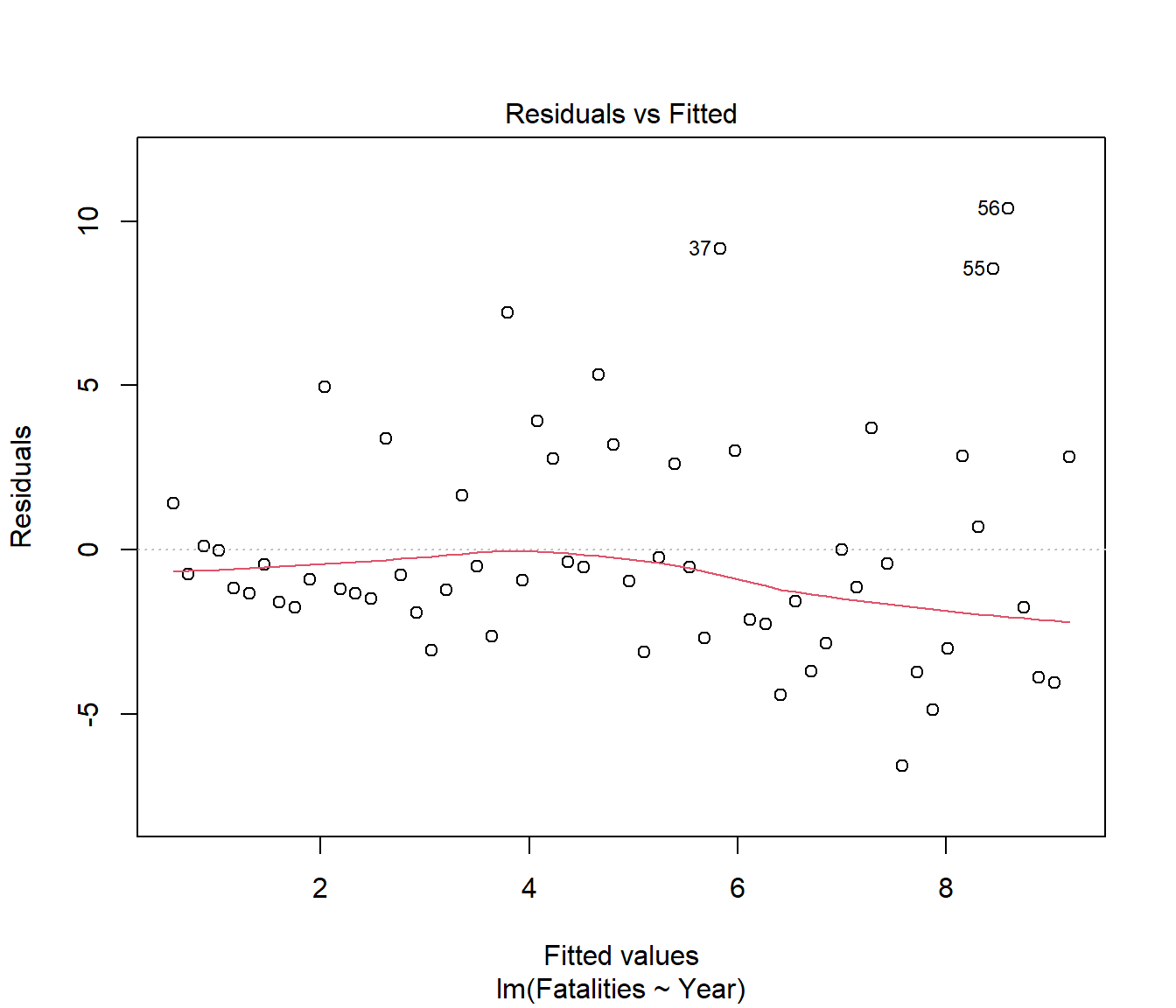
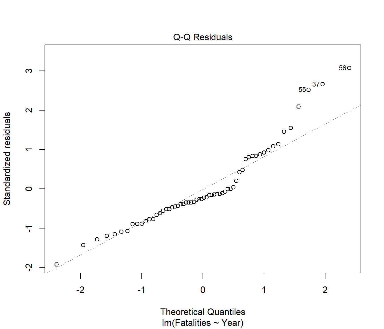
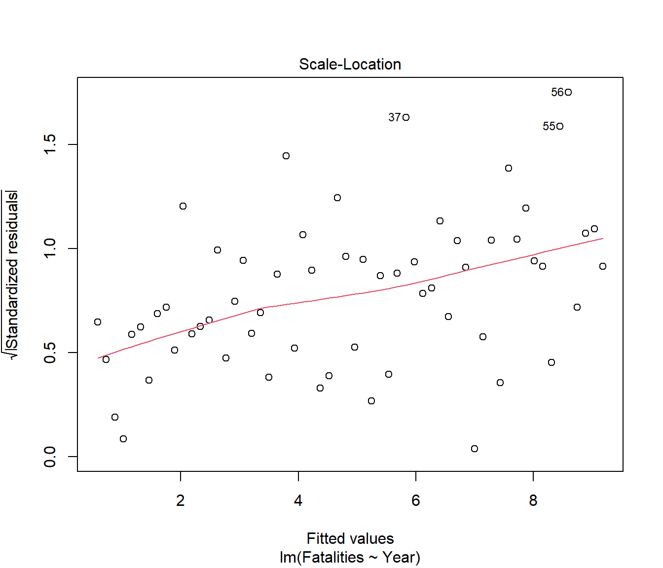
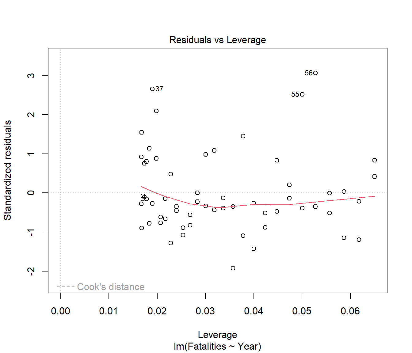
We see that the spread of residuals has been increasing. This has carried through to affect the normality in the residuals.
What about curvature? This is more subtle because it looks as if the straight-line model is fine, but your eye does not take into account the fact that there is a lower bound on the Y-values: there cannot be negative numbers of Fatalities.
Now the fitted line does not go negative, so there is no problem, right?
Wrong. A statistical model is not just about the fitted line, but about modelling the whole data, including understanding the errors or variation around the line. The constant variance assumption implies that we should be able to see (roughly) the same spread of errors above and below the regression line all the way along the x-axis.
This is illustrated by the following ‘prediction interval’ graph which indicates we should expect to be able to get data all through the shaded area which is roughly \(\hat{y} \pm 2 S\) where S is the residual standard error (we will see in the next topic how exactly this graph is created).
One way to get a shaded area which stays above zero is to try a transformation, which will also reduce the distance between the bounds at the left, perhaps something like this -
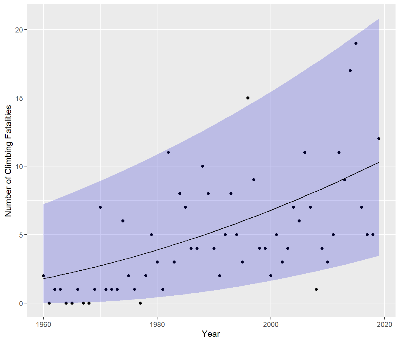
OK, that made it better, but we have not totally eliminated the problem associated with estimation near the boundary value of zero fatalities.
7.8 What sort of transformation should we choose?
If the response variable Y is bounded below (e.g. negatives are impossible) and right-skewed (tending to high positive outliers) then common transformations are sqrt(Y) and log(Y). Sometimes sqrt(Y+1) or log(Y+1) is used to improve the fit, especially if some Y=0 (one cannot take log of 0). The graph above was fitted using the linear model \[ Y_{new} = \beta_0 + \beta_1 \hbox{Year} + \varepsilon\] where \(Y_{new} = \log{\hbox{Fatalities}+1}\). This is still regarded as a linear model since the \(\beta\)s are separated by plusses.
The fitted line has then been back-transformed to the original scale, hence it has become a curve, which can be written as \[ \hat{y} = \exp\left( \hat{\beta_0} + \hat{\beta_1} \hbox{Year} \right) -1 .\]
7.8.1 Is the transformation suitable?
In one sense the graph above answers the question: the shaded area seems to fit the data quite well. But the proper answer is to look at the residuals in the transformed (\(Y_{new}\)) units.
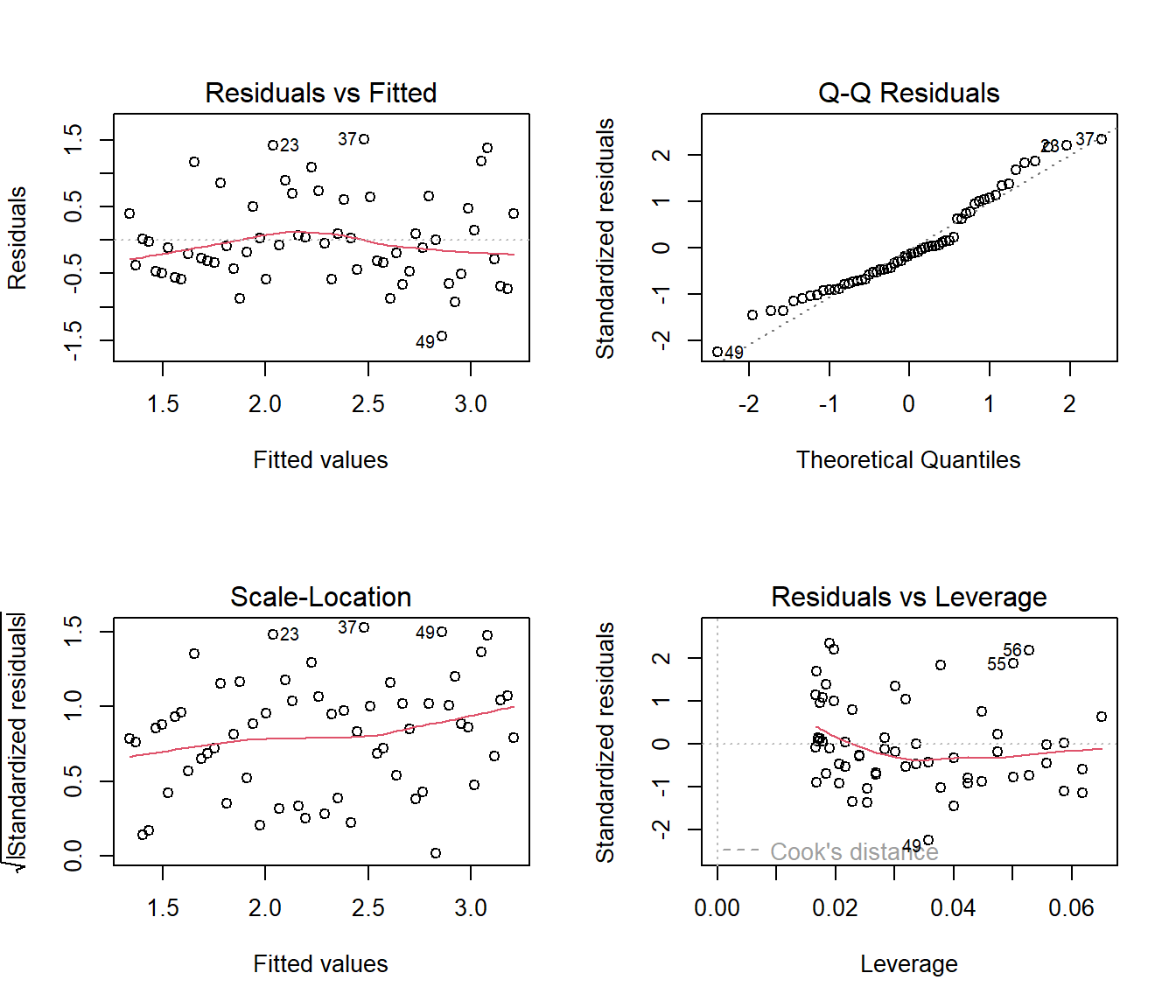
It looks like the heteroscedasticity (A3) and normality (A4) have been improved, and there is no problem with curvature (A1). Less of the graph in the original units goes into impossible territory. So the model appears somewhat useful even if it isn’t perfect.
7.8.2 What is the justification for this transformation?
There is some maths behind why square root and log are common transformations, especially for data consisting of counted occurrences, but the reasoning will have to be left to another course. For our purposes, we just look for a transformation that fixes the residuals on the transformed scale. Then for prediction we back-transform the result. You can read more about transformation methods in an Appendix to this book of notes.
The course 161.331 considers something called Generalized Linear Models, which are a class of regression models used when the response variable \(Y\) does not have normal errors. Many of the techniques you will learn in 161.251 generalize easily into that wider variety of contexts.