Lecture 8 Prediction in Simple Linear Regression
This lecture will cover prediction for (Simple) Linear Regression. Extending the ideas to more complicated models follows a relatively easy modification to the process.
8.1 Prediction from Regression Models
Simple linear regression models can be used to predict the response at any specified value of the predictor.
Nonetheless, we should beware predicting far beyond the range of the data.
Point predictions should be accompanied by corresponding prediction intervals, providing a range of plausible values.
8.2 The Basics of Prediction
Suppose that we want to predict the response when the predictor x takes the specific value x0, a value not necessarily seen in the observed data. N.B. The use of the zero in the subscript relates to the specific observation; you might ignore it for clarity.
We denote the prediction by \(\hat{y_0}\), called “y hat”. The subscript links this prediction to the specific x value denoted x0. If we were doing this prediction for the observed data, we could use the subscript i in these expressions.
Our model for the corresponding response, y0, is
\[Y_0 = \mu_0 + \varepsilon_0\] where \[\mu_0 = \beta_0 + \beta_1 x_0\]
It is natural to estimate \(\mu_0\) by
\[\hat \mu_0 = \hat \beta_0 + \hat \beta_1 x_0\]
We have no information about \(\varepsilon_0\) so it is estimated by its expected value. i.e. we define \(\hat \varepsilon_0 = 0\) as the estimate of \(\varepsilon_0\).
Then \[\begin{aligned} \hat y_0 &=& \hat \mu_0 + \hat \varepsilon_0\\ &=& \hat \beta_0 + \hat \beta_1 x_0\end{aligned}\]
This should be fairly intuitive — we just read the prediction from the fitted regression line.
8.3 Prediction Versus Estimation of Mean Response
The prediction was \(\hat y_0 = \hat \mu_0\)
But \(\hat \mu_0\) is also the natural estimate of \(\mu_0 = E[Y_0]\).
Hence the prediction is the same as the estimate of the mean response.
However, differences arise if we want to construct corresponding interval estimates.
8.4 Confidence Interval for the Mean Response
The standard deviation of the sampling distribution of \(\hat \mu_0\) is
\[\sigma_{\hat\mu_0} = \sigma \sqrt{ \frac1n + \frac{ (x_0 - \bar x)^2} {s_{xx}} }\]
The standard error for \(\hat \mu_0\) is
\[SE(\hat \mu_0) = s \sqrt{ \frac1n + \frac{(x_0 - \bar x)^2} {s_{xx}} } \; .\]
It can be shown that the sampling distribution of \(\hat \mu_0\) is defined by
\[\frac{ \hat \mu_0 - \mu_0 }{SE(\hat \mu_0)} \sim t(n-2)\]
Hence a \(100(1-\alpha)\%\) confidence interval for \(\mu_0\) is given by
\[\left ( \hat \mu_0 - t_{\alpha/2} SE(\hat \mu_0), \; \hat \mu_0 + t_{\alpha/2} SE(\hat \mu_0) \right )\]
where \(t_{\alpha/2}\) is a critical value from the t distribution with df=n-2.
This confidence interval provides a range of plausible values for the mean response \(\hat \mu_0\) and the interval gets narrower as we gather larger samples. In practice we will not need to use these formulas: R will produce the confidence intervals for us.
8.5 Prediction Intervals
When it comes to finding the prediction error for y0, we must take into account the additional variation among individuals expressed by the \(\varepsilon_0\) term:
\[\mbox{var}(\hat{y_0}) = \mbox{var}(\hat{\mu_0}) + \mbox{var}(\varepsilon_0) = [SE(\hat{\mu_0})]^2 + \sigma^2\]
Replacing \(\sigma^2\) by its estimate s2, we get the prediction error of \(\hat y_0\) as
\[PE(\hat y_0) = s \sqrt{ \frac1n + \frac{(x_0 - \bar{x})^2}{s_{xx} }+1} \; .\]
A \(100(1-\alpha)\%\) prediction interval for y0 is then
\[\left ( \hat{y_0} - t_{\alpha/2} PE(\hat{y_0}), \; \hat{y_0} + t_{\alpha/2} PE(\hat y_0) \right )\]
As the name suggests, the probability that y0 will actually lie in this prediction interval is \(1-\alpha\).
Again, we will not need to calculate these intervals by hand: R will do it for us. To get the predicted values we set \(x_0\) (which can be more than one value) in an object called a data.frame, then invoke the predict() function based on an existing linear model.
8.6 Boiling Point Data
We will use data on boiling point in degrees Fahrenheit (y) and pressure in inches of mercury (x), collected during an expedition in the Alps.
Data source: A Handbook of Small Data Sets by Hand, Daly, Lunn, McConway and Ostrowski; also known as forbes in the `MASS package.

8.6.1 Prediction for Boiling Point Data in R
## Boil <- read.csv(file = "https://r-resources.massey.ac.nz/data/161251/boiling.csv",
##     header = TRUE)
Boil.lm <- lm(BPt ~ Pressure, data = Boil)
summary(Boil.lm)
Call:
lm(formula = BPt ~ Pressure, data = Boil)

Residuals:
     Min       1Q   Median       3Q      Max
-1.22687 -0.22178  0.07723  0.19687  0.51001

Coefficients:
             Estimate Std. Error t value Pr(>|t|)
(Intercept) 155.29648    0.92734  167.47   <2e-16 ***
Pressure      1.90178    0.03676   51.74   <2e-16 ***
---
Signif. codes:  0 '***' 0.001 '**' 0.01 '*' 0.05 '.' 0.1 ' ' 1

Residual standard error: 0.444 on 15 degrees of freedom
Multiple R-squared:  0.9944,    Adjusted R-squared:  0.9941
F-statistic:  2677 on 1 and 15 DF,  p-value: < 2.2e-16
x0 <- data.frame(Pressure = c(27, 32))
predict(Boil.lm, newdata = x0, interval = "prediction", level = 0.95) fit lwr upr
1 206.6446 205.6590 207.6303
2 216.1536 215.0382 217.2690We can use the predict() function (with one small change) to obtain the confidence intervals for the mean response at the same values of the predictor using:
       fit      lwr      upr
1 206.6446 206.3693 206.9200
2 216.1536 215.5633 216.7438
8.6.2 Fitted Line Plot for Boiling Point Data
ggplot(Boil, mapping = aes(y = BPt, x = Pressure)) + geom_point() + geom_smooth(method = "lm",
    se = FALSE) + ylab("Boiling Point") + xlab("Pressure")
`geom_smooth()` using formula = 'y ~ x'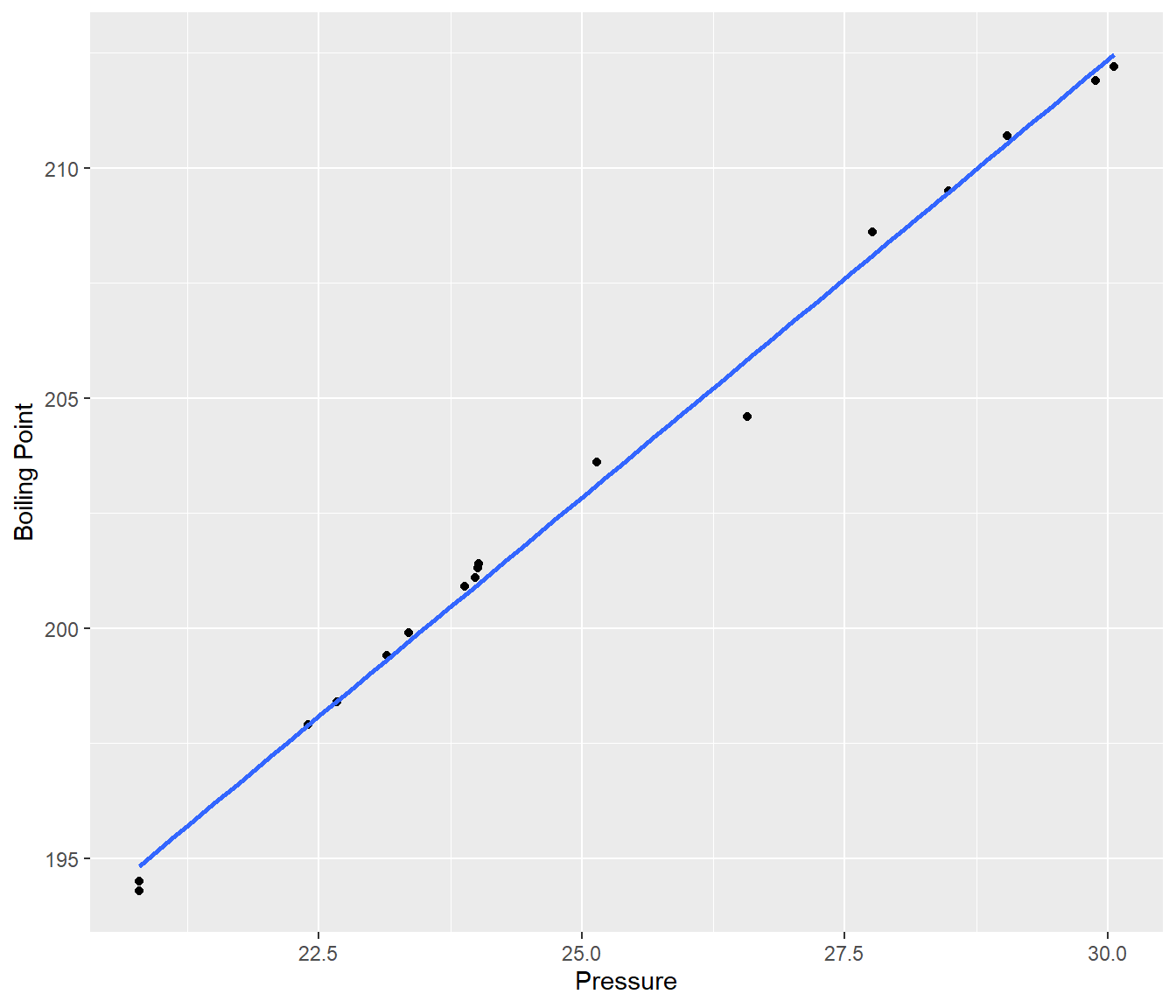
The model fit looks good so we should expect fairly tight prediction intervals.
8.7 Conclusions for Boiling Point Data
Fitted model is \[E[\mbox{BPt}] = 155.3 + 1.902~\mbox{Pressure}\]
Pressure explains over 99% of the variation in boiling point.
When pressure is 27 inches of mercury, predicted temperature is 206.6 degrees Fahrenheit with 95% prediction interval (205.7, 207.6).
When pressure is 32 inches of mercury, prediction is 216.2 with 95% prediction interval (215.0, 217.3).
8.8 Test your understanding
Use the model above to prove to yourself that:
- The prediction interval is wider than the confidence interval for a given x0.
- the intervals get wider the farther x0 gets from \(\bar{x}\).
- the intervals get wider when the level of confidence for the interval increases.
x0 <- data.frame(Pressure = c(27:32))
predict(Boil.lm, newdata = x0, interval = "prediction", level = 0.95)
fit lwr upr
1 206.6446 205.6590 207.6303
2 208.5464 207.5457 209.5472
3 210.4482 209.4266 211.4698
4 212.3500 211.3020 213.3980
5 214.2518 213.1724 215.3312
6 216.1536 215.0382 217.2690 fit lwr upr
1 206.6446 206.3693 206.9200
2 208.5464 208.2212 208.8717
3 210.4482 210.0635 210.8329
4 212.3500 211.8999 212.8000
5 214.2518 213.7328 214.7707
6 216.1536 215.5633 216.7438 fit lwr upr
1 206.6446 206.2640 207.0253
2 208.5464 208.0968 208.9961
3 210.4482 209.9163 210.9801
4 212.3500 211.7278 212.9722
5 214.2518 213.5343 214.9693
6 216.1536 215.3375 216.9696