Lecture 19 Linear Models with One Factor
So far we have focused on regression models, where a continuous random response variable is modelled as a function of one or more numerical explanatory variables.
Another common situation is where the explanatory variables are categorical variables, or what we will often call factors.
In this lecture we will begin to look at such models, and will focus in particular on one-way models.
19.1 The One-Way Model
The one-way (or one factor) model is used when a continuous numerical response Y is dependent on a single factor (categorical explanatory variable).
In such models, the categories defined by a factor are called the levels of the factor.
19.2 Stimulating Effects of Caffeine
Question: does caffeine stimulation affect the rate at which individuals can tap their fingers?
Thirty male students randomly allocated to three treatment groups of 10 students each. Groups treated as follows:
Group 1: zero caffeine dose
Group 2: low caffeine dose
Group 3: high caffeine dose
Allocation to treatment groups was blind (subjects did not know their caffeine dosage).
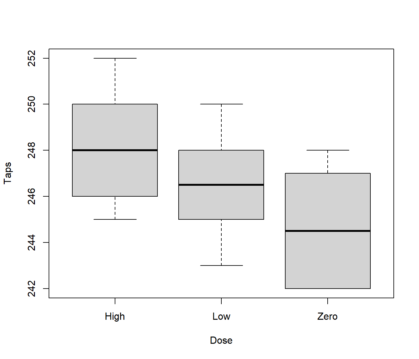
Two hours after treatment, each subject tapped fingers as quickly as possible for a minute. Number of taps recorded.
Number of taps is the response variable, caffeine dose is the explanatory variable. Here caffeine dose is a factor with 3 levels - zero, low and high. Does apparent trend in boxplot provide convincing evidence that caffeine affects tapping rate?
19.3 Mathematical Formulation of the One-Way Model
It is common to express the One-way model as
\[y_{ij} = \mu_j + \varepsilon_{ij}~~~~~~~~(j=1,\ldots,K,~~~~~i=1,\ldots,n_j)\]
where: yij is the response of the ith unit at the jth level of the factor; K denotes the number of levels; \(\mu_j\) is the (unknown) population mean for level \(j\)
nj the number of observations (replications) at level j of the factor; and, the values \(\varepsilon_{11},..,\varepsilon_{Kn_K}\) are random errors satisfying assumptions (A1)-(A4)
The null hypothesis is then expressed as
\[H_0: ~~~ \mu_1 = \mu_2 = ... =\mu_K \] and the alternative hypothesis is
\[H_1: ~~~\mbox{ means not all equal.}\]
Another way of writing this is \[y_{ij} = \mu + \alpha_j + \varepsilon_{ij}~~~~~~~~(j=1,\ldots,K,~~~~~i=1,\ldots,n_i)\]
where \(\alpha_j = \mu_j - \mu\) (mean difference to the baseline) for \(j=1,...,K\).
The mean response is \[E[Y_{ij}] = \mu + \alpha_j\]
19.4 Parameterisation of the One-Way Model
However, as it stands, the model appears to be overparameterised.
That is, we have \(K\) means and we are trying to estimate K+1 parameters \(\mu,\alpha_1,...,\alpha_K\)
We cannot estimate K+1 numbers from k bits of information.
19.5 Solution to Overparameterisation
We impose a constraint on the parameters \(\alpha_1, \alpha_2, \ldots, \alpha_K\).
The two most popular (and easily interpretable) constraints are:
Sum constraints: \(\sum_{j=1}^K \alpha_j = 0\).
In this case \(\mu\) can be interpreted as a kind of “grand mean”, and \(\alpha_1, \alpha_2, \ldots, \alpha_K\) measure deviations from this grand mean.Treatment constraint: \(\alpha_1 = 0\).
In this case level 1 of the factor is regarded as the baseline or reference level, and \(\alpha_2, \alpha_3 \ldots, \alpha_K\) measure deviations from this baseline. This is highly appropriate if level 1 corresponds to a control group, for example.
We will work with the treatment constraint. It is also used by default for factors in R.
19.6 Expressing Factor Models as Regression Models
We can express a one-way factor model as a regression model by using dummy (indicator) variables.
Define dummy variables \(z_{11}, z_{12}, \ldots, z_{n K}\) by \[z_{ij} = \left \{ \begin{array}{ll} 1 & \mbox{unit i observed at factor level j}\\ 0 & \mbox{otherwise.} \end{array} \right .\]
19.7 Regression form of one-way factor model
A one-way factor model can be expressed as follows: \[y_i = \mu + \alpha_1 z_{i1} + \alpha_2 z_{i2} + \ldots + \alpha_K z_{iK} + \varepsilon_i~~~~~(i=1,2,\ldots,n)\]
This has the form of a multiple linear regression model.
The parameter \(\mu\) is the regression intercept and, under the treatment constraint (\(\alpha_1 = 0\)), the mean baseline (factor level 1) response.
19.8 Modelling the Caffeine Data
Our one-way factor model, where the factor has three levels, can be expressed as follows: \[y_i = \mu + \alpha_2 z_{i2} + \alpha_{3} z_{i3} + \varepsilon_i\]
where: yi is the number of taps recorded for the ith subject; zi2 = 1 if subject i is on low dose; zi2 = 0 otherwise; and zi3 = 1 if subject i is on high dose; zi3 = 0 otherwise.
Then, \(\mu\) is mean response for a subject on zero dose; \(\alpha_2\) is the effect of low dose in contrast to zero dose; and, \(\alpha_3\) is the effect of high dose in contrast to zero dose.
19.9 Expressing Factorial Models using Matrices
Since factorial models can be expressed as linear regression models, they may be described using matrix notation as we saw earlier.
For a one-way factorial model with treatment constraint: \[{\boldsymbol{y}} = X {\boldsymbol{\beta}} + \varepsilon\] where: \[{\boldsymbol{y}} = \left [ \begin{array}{c} Y_1\\ Y_2\\ \vdots\\ Y_n \end{array} \right ] ~~~~X = \left [ \begin{array}{cccc} 1 & z_{12} & \ldots & z_{1K}\\ 1 & z_{22} & \ldots & z_{2K}\\ \vdots & \vdots & \ddots & \vdots\\ 1 & z_{n2} & \ldots & z_{nK} \end{array} \right ] ~~~ {\boldsymbol{\beta}} = \left [ \begin{array}{c} \mu\\ \alpha_2\\ \vdots\\ \alpha_K\\ \end{array} \right ] ~~~ \boldsymbol{\varepsilon} = \left [ \begin{array}{c} \varepsilon_1\\ \varepsilon_2\\ \vdots\\ \varepsilon_n\\ \end{array} \right ]\]
There is no \(\alpha_1\) in the parameter vector, and no row for \(z_{i1}\) in the design matrix, because of the treatment constraint.
The following shows the design matrix for the one-way model for the caffeine data.
| (Intercept) | DoseLow | DoseZero |
|---|---|---|
| 1 | 0 | 1 |
| 1 | 0 | 1 |
| 1 | 0 | 1 |
| 1 | 0 | 1 |
| 1 | 0 | 1 |
| 1 | 0 | 1 |
| 1 | 0 | 1 |
| 1 | 0 | 1 |
| 1 | 0 | 1 |
| 1 | 0 | 1 |
| 1 | 1 | 0 |
| 1 | 1 | 0 |
| 1 | 1 | 0 |
| 1 | 1 | 0 |
| 1 | 1 | 0 |
| 1 | 1 | 0 |
| 1 | 1 | 0 |
| 1 | 1 | 0 |
| 1 | 1 | 0 |
| 1 | 1 | 0 |
| 1 | 0 | 0 |
| 1 | 0 | 0 |
| 1 | 0 | 0 |
| 1 | 0 | 0 |
| 1 | 0 | 0 |
| 1 | 0 | 0 |
| 1 | 0 | 0 |
| 1 | 0 | 0 |
| 1 | 0 | 0 |
| 1 | 0 | 0 |
19.10 Factor Models as Regression Models
Since factor models can be regarded as regression models, all ideas about parameter estimation, fitted values etc. follow in the natural manner.
Parameter estimation can be done by the method of least squares, to give vector of estimates \(\hat {\boldsymbol{\beta}} = (\hat \mu, \hat \alpha_2, \ldots, \hat \alpha_K)^T\).
Fitted values and residuals defined in the usual way.
19.11 Back to the Caffeine Data
19.11.1 R Code
The factor levels of Dose have a natural ordering. In particular, it is intuitive to set the zero level as baseline (factor level 1).
'data.frame':   30 obs. of  2 variables:
 $ Taps: int  242 245 244 248 247 248 242 244 246 242 ...
$ Dose: chr "Zero" "Zero" "Zero" "Zero" ... Taps Dose
1 242 Zero
2 245 Zero
3 244 Zero
4 248 Zero
5 247 Zero
6 248 Zero
7 242 Zero
8 244 Zero
9 246 Zero
10 242 Zero
11 248 Low
12 246 Low
13 245 Low
14 247 Low
15 248 Low
16 250 Low
17 247 Low
18 246 Low
19 243 Low
20 244 Low
21 246 High
22 248 High
23 250 High
24 252 High
25 248 High
26 250 High
27 246 High
28 248 High
29 245 High
30 250 HighWe fix up the order of the factor levels (default is alphabetical).
NULL[1] "Zero" "Low" "High"The syntax using the factor() command (with specified levels) reorders
the factor levels so that zero, low and high dose are interpreted as
levels 1, 2 and 3 respectively.
Fitting the Model
We can use the lm() function in R to fit model
in the same manner as for regression models.
Call:
lm(formula = Taps ~ Dose, data = Caffeine)

Residuals:
   Min     1Q Median     3Q    Max
-3.400 -2.075 -0.300  1.675  3.700

Coefficients:
            Estimate Std. Error t value Pr(>|t|)
(Intercept) 244.8000     0.7047 347.359  < 2e-16 ***
DoseLow       1.6000     0.9967   1.605  0.12005
DoseHigh      3.5000     0.9967   3.512  0.00158 **
---
Signif. codes:  0 '***' 0.001 '**' 0.01 '*' 0.05 '.' 0.1 ' ' 1

Residual standard error: 2.229 on 27 degrees of freedom
Multiple R-squared:  0.3141,    Adjusted R-squared:  0.2633
F-statistic: 6.181 on 2 and 27 DF,  p-value: 0.006163
Using the notation introduced earlier, the parameter estimates are \(\hat \mu = 244.8\), \(\hat \alpha_2 = 1.6\) and \(\hat \alpha_3 = 3.5\).
19.12 fitted values
| Dose (level) | mean response | fitted value |
|---|---|---|
| Zero (1) | \(\mu\) | 244.8 |
| Low (2) | \(\mu + \alpha_2\) | 246.4 |
| High (3) | \(\mu + \alpha_3\) | 248.3 |
19.13 Hypothesis tests
There are three ways we can think of the hypothesis test.
The first formulation of the model (with \(H_0: ~~~ \mu_1 = \mu_2 = ... =\mu_K\)) can be tested by just looking at the \(F\) test at the bottom of the summary(lm) output, or applying the anova() command to the output.
Analysis of Variance Table

Response: Taps
          Df Sum Sq Mean Sq F value   Pr(>F)
Dose       2   61.4 30.7000  6.1812 0.006163 **
Residuals 27  134.1  4.9667
---
Signif. codes:  0 '***' 0.001 '**' 0.01 '*' 0.05 '.' 0.1 ' ' 1
On the other hand writing the Factor models (using the treatment constraint) can be written as multiple linear regression models, using dummy variables:
\[Y_i = \mu + \alpha_2 z_{i2} + \ldots + \alpha_K z_{iK} + \varepsilon_i \quad(i=1,2,\ldots,n)\]
we can regard the F test as testing the hypothesis that all slopes are zero \(H_0: \alpha_2 = ...=\alpha_K = 0\), which gives the same omnibus F test.
z2 = Caffeine$Dose == "Low"
z3 = Caffeine$Dose == "High"
Caffeine.lm2 = lm(Caffeine$Taps ~ z2 + z3)
summary(Caffeine.lm2)
Call:
lm(formula = Caffeine$Taps ~ z2 + z3)

Residuals:
   Min     1Q Median     3Q    Max
-3.400 -2.075 -0.300  1.675  3.700

Coefficients:
            Estimate Std. Error t value Pr(>|t|)
(Intercept) 244.8000     0.7047 347.359  < 2e-16 ***
z2TRUE        1.6000     0.9967   1.605  0.12005
z3TRUE        3.5000     0.9967   3.512  0.00158 **
---
Signif. codes:  0 '***' 0.001 '**' 0.01 '*' 0.05 '.' 0.1 ' ' 1

Residual standard error: 2.229 on 27 degrees of freedom
Multiple R-squared:  0.3141,    Adjusted R-squared:  0.2633
F-statistic: 6.181 on 2 and 27 DF,  p-value: 0.006163
Finally we can consider the problem as a comparison of two models
\[M0:~~~~ Y_i = \mu + \varepsilon_i \quad (i=1,2,\ldots,n)\] and \[M1:~~~~ Y_i = \mu + \alpha_2 z_{i2} + \ldots + \alpha_K z_{iK} + \varepsilon_i \quad (i=1,2,\ldots,n)\] Thus
Caffeine.M0 = lm(Caffeine$Taps ~ 1)
Caffeine.M1 = lm(Caffeine$Taps ~ z2 + z3)
anova(Caffeine.M0, Caffeine.M1)
Analysis of Variance Table
Model 1: Caffeine$Taps ~ 1
Model 2: Caffeine$Taps ~ z2 + z3
Res.Df RSS Df Sum of Sq F Pr(>F)
1 29 195.5
2 27 134.1 2 61.4 6.1812 0.006163 **
---
Signif. codes: 0 '***' 0.001 '**' 0.01 '*' 0.05 '.' 0.1 ' ' 1Important:
- In a multiple linear regression model it makes sense to add or remove a single explanatory variable.
- In a factor model it (usually) only makes sense to add or remove a whole factor, not single levels of a factor.
- This will usually require F tests (not just t-tests for single parameters).
19.13.0.1 Conclusions from the ANOVA table
The observed F-statistic for testing for the significance of caffeine dose is f = 6.181 on K-1 = 2 and n-K = 27 degrees of freedom.
The corresponding P-value is P=0.0062; we therefore have very strong evidence against H0; i.e. finger tapping speed does seem to be related to caffeine dose.
The table of coefficients in the R output shows that the mean response difference between the high dose and control groups is a little more than twice as big as the difference between low dose and control group.
19.13.1 Interpretation of the anova output
Use the anova output produced by R to answer the following questions on the caffeine data.
What is the residual sum of squares for the full model M1?
What is the mean sum of squares for the model M1?
What is the residual sum of squares for the null model M0, given below? \[M0: Y_i = \mu + \varepsilon_i~~~~~~~(i=1,2,\ldots,30)\]
What is the mean sum of squares for the model M0?