Lecture 34 Models with Autoregressive Errors
We saw previously that when linear models are fitted to time series data, the residuals can display autocorrelation. The consequences of autocorrelation are that
standard errors given by standard least squares theory (and hence by standard R output) will usually be smaller than the true standard deviations of the parameter estimates.
the result is that t-test statistics will be inflated, p-values too small, and confidence intervals will be too narrow.
34.1 Accounting for Autocorrelation in the Errors
The consequence of standard errors and p-values being out means that we need to account for autocorrelation in the errors when it is present.
This will require two steps:
- Definition of an appropriate model for autocorrelated errors;
- Fitting the linear model with autocorrelated errors.
We now consider modeling the errors using autoregressive models.
34.2 Autoregressive Models
In a time series, the errors \(\varepsilon_1, \varepsilon_2, \ldots, \varepsilon_n\) can be thought of as a realization of a random process (in time).
We can model serial correlation between these errors by making each one explicitly dependent on the previous one: \[\varepsilon_t = \phi \varepsilon_{t-1} + \eta_t\] where \(\eta_t~(t=1,2,\ldots,n)\) is white noise, that is, a sequence of independent and identically distributed (normal) random variables with zero mean.
- This equation is a first order autoregressive (or AR1) model for \(\varepsilon_t\).
- Under this model, \(\mbox{Corr}(\varepsilon_t, \varepsilon_{t-1}) = \phi\).
- Consequently, more generally, \(\mbox{Corr}(\varepsilon_t, \varepsilon_{t-k}) = \phi^k\)
34.3 ACF Plots for AR1 Processes
To illustrate an ACF plot for a function demonstrating autocorrelation, we create two variables from white noise
Z1 = rnorm(1000)
X1 = Z1[-1] + 0.85 * Z1[-1000]
X2 = Z1[-1] - 0.85 * Z1[-1000]
par(mfrow = c(1, 2), mai = rep(0.5, 4))
plot(X1, type = "l")
plot(X2, type = "l")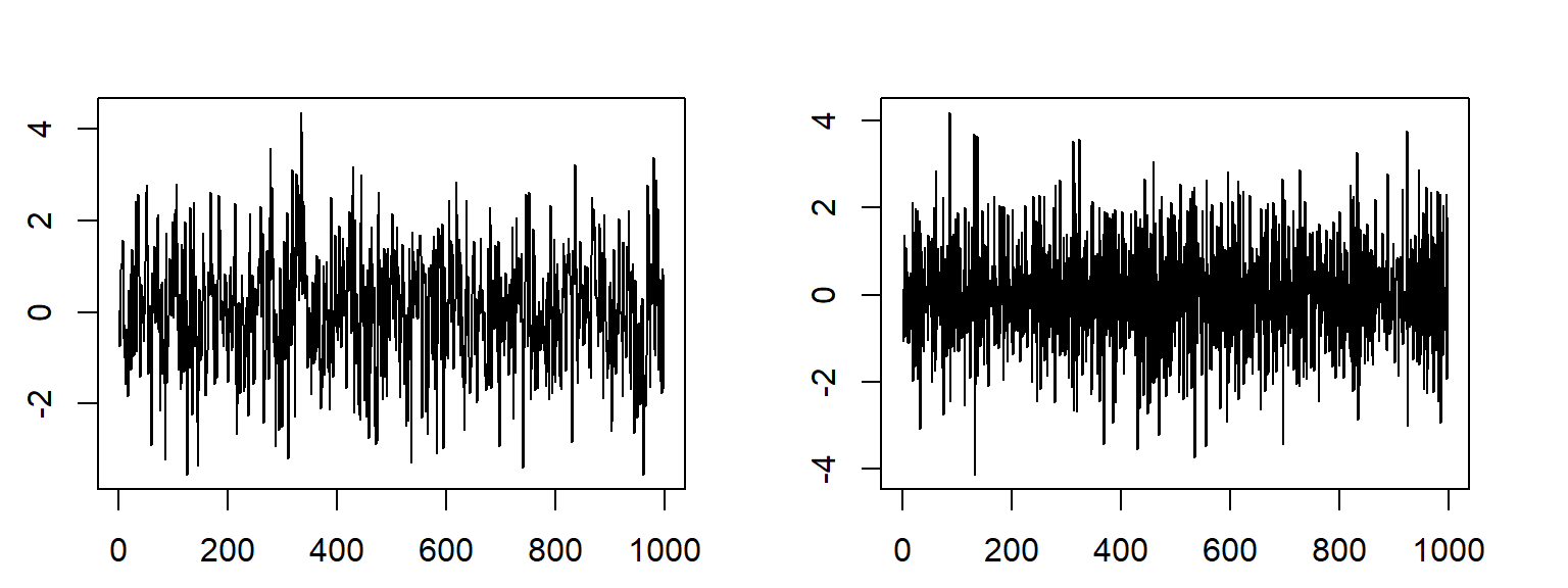
34.4
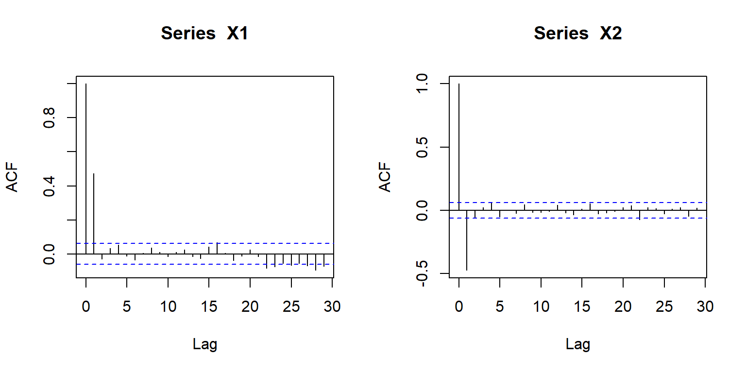
The X1 series has correlation of 0.457 at lag 1, while the X2 series has autocorrelation of -0.504 at lag1
34.5 Autoregressive Models for Errors in Linear Modelling
If residuals in a linear model for time series data display autocorrelation then we change the model to allow for an AR1 correlation structure for the residuals in our model to account for this.
N.B. More complex models are also possible. For example:
- AR models of order q>1, where \(\varepsilon_t\) is modelled as explicitly dependent on the previous q errors;
- moving average (MA) models and autoregressive moving average (ARMA) models.
- For the purposes of this course we will focus on AR1 models for the error process.
34.6 Application to the Tourism Data
## tourism <- read_csv(file = "motel.csv")
tourism <- tourism |>
    mutate(Time = round(time_length(Date - min(Date), unit = "month")), Month = factor(month(Date,
        label = TRUE), ordered = FALSE), Year = year(Date))
tourism
# A tibble: 180 × 6
Date RoomNights AvePrice Time Month Year
<date> <dbl> <dbl> <dbl> <fct> <dbl>
1 1980-01-01 276986 27.7 0 Jan 1980
2 1980-02-01 260633 28.7 1 Feb 1980
3 1980-03-01 291551 28.6 2 Mar 1980
4 1980-04-01 275383 28.3 3 Apr 1980
5 1980-05-01 275302 28.7 4 May 1980
6 1980-06-01 231693 28.6 5 Jun 1980
7 1980-07-01 238829 29.2 6 Jul 1980
8 1980-08-01 274215 29.8 7 Aug 1980
9 1980-09-01 277808 29.6 8 Sept 1980
10 1980-10-01 299060 30.3 9 Oct 1980
# ℹ 170 more rows34.7
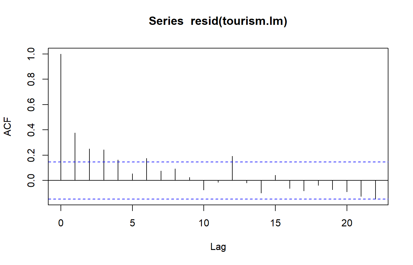
There is a suggestion of exponential decay in autocorrelations. - AR1 model (with positive \(\phi\)) for errors seems reasonable.
34.8
The model incorporating the AR1 error process, and written in regression format, is as follows:
\[\begin{aligned} Y_{t} &= \beta_0 + \beta_1 \mbox{Time} + \beta_2 z_{t,2} + \beta_3 z_{t,3} + \ldots + \beta_{12} z_{t,12} + \varepsilon_t \\ \varepsilon_t &= \phi \varepsilon_{t-1} + \eta_{t}\end{aligned}\]
where:
- \(Y_t\) is the \(t\)th observation of
RoomNights; - \(z_{t,j} = 1\) if observation \(t\) is taken in month \(j\);
- \(z_{t,j} = 0\) otherwise.
- \(\eta_1, \ldots, \eta_n\) are independent and identically distributed normal random variables with mean zero.
34.9 Model Fitting with Autoregressive Errors
To fit a model with AR1 errors, we must:
- Estimate the size of the autocorrelation parameter, \(\phi\).
- Account for the autocorrelation in errors when estimating the regression coefficients.
The AR1 parameter, \(\phi\), can be estimated by the method of (restricted) maximum likelihood.
The details are beyond the scope of this paper, but you will meet maximum likelihood estimation if you take 161.304 or 161.331.
Once \(\phi\) is estimated, we can account for the AR1 nature of the errors by fitting the linear model using generalized least squares.
34.10 Generalized Least Squares
Once we have \(\phi\) estimated, we can then estimate the regression coefficients \(\beta\) by rearranging the regression equation to eliminate the autocorrelation:
Suppose \[ \begin{aligned} y_t &= \beta_0 + \beta_1 x_t + \varepsilon_t\\ \varepsilon_t &= \phi \varepsilon_{t-1} + \eta_t \end{aligned} \] where \(\eta_t \underset{\mathsf{iid}}\sim N(0, 1)\). Then \[ \begin{aligned} y_t - \phi y_{t-1} &= \beta_0 + \beta_1 x_t + \varepsilon_t - \phi (\beta_0 + \beta_1 x_{t-1} + \varepsilon_{t-1})\\ &= \beta_0(1 - \phi) + \beta_1 (x_t - \phi x_{t-1}) + \varepsilon_t - \phi \varepsilon_{t-1}\\ &= \beta_0(1 - \phi) + \beta_1 (x_t - \phi x_{t-1}) + \eta_t \end{aligned} \] which is a standard linear regression in the new variables \(Y_t = y_t - \phi y_{t-1}\), \(X_t = x_t - \phi x_{t-1}\).
Thus we can fit this with least squares. The “generalised” bit is the trick we use to transform something that is not regular least squares to a least squares situation - it turns out we can do this no matter what the covariance structure is among the predictors as long as the structure is estimable from the data.
34.11 Generalized Least Squares in R
In R, linear models can be fitted using this technique using the gls() command found in the nlme add-on package.
Call this package using library(nlme) before using the gls() command.
- The
gls()command uses the same model formula aslm(), but also accepts an additional argument to describe the correlation structure for the errors.
34.12 Generalized Least Squares and the Tourism Data
tourism.gls <- gls(RoomNights ~ Time + Month, correlation = corAR1(), data = tourism)
anova(tourism.gls)
Denom. DF: 167
numDF F-value p-value
(Intercept) 1 45239.15 <.0001
Time 1 1092.85 <.0001
Month 11 81.94 <.0001The use of an AR1 error process is obtained by setting correlation=corAR1() in the gls() command.
Both Time and Month are associated with
RoomNights (P-value less than \(0.0001\) in both
cases).
34.13
Generalized least squares fit by REML
  Model: RoomNights ~ Time + Month
  Data: tourism
       AIC      BIC    logLik
  3727.911 3774.681 -1848.955

Correlation Structure: AR(1)
 Formula: ~1
 Parameter estimate(s):
     Phi
0.392721

Coefficients:
                Value Std.Error   t-value p-value
(Intercept) 275492.20  4692.407  58.71021  0.0000
Time          1062.25    31.870  33.33115  0.0000
MonthFeb    -31194.09  4205.044  -7.41825  0.0000
MonthMar     23482.73  4959.531   4.73487  0.0000
MonthApr     -2170.47  5225.494  -0.41536  0.6784
MonthMay    -19419.12  5325.710  -3.64630  0.0004
MonthJun    -65827.11  5362.987 -12.27434  0.0000
MonthJul    -44522.34  5373.207  -8.28599  0.0000
MonthAug    -29768.74  5365.559  -5.54812  0.0000
MonthSept   -12039.27  5331.948  -2.25795  0.0252
MonthOct     26393.95  5238.620   5.03834  0.0000
MonthNov     16471.67  4988.022   3.30224  0.0012
MonthDec    -58631.94  4272.401 -13.72342  0.0000

 Correlation:
          (Intr) Time   MnthFb MnthMr MnthAp MnthMy MnthJn MnthJl MnthAg MnthSp
Time      -0.586
MonthFeb  -0.447  0.003
MonthMar  -0.525 -0.001  0.589
MonthApr  -0.551 -0.005  0.462  0.659
MonthMay  -0.558 -0.011  0.416  0.535  0.682
MonthJun  -0.559 -0.016  0.398  0.487  0.560  0.690
MonthJul  -0.557 -0.022  0.391  0.468  0.512  0.568  0.692
MonthAug  -0.552 -0.028  0.387  0.460  0.492  0.520  0.571  0.692
MonthSept -0.545 -0.034  0.383  0.454  0.481  0.498  0.520  0.569  0.690
MonthOct  -0.532 -0.039  0.376  0.445  0.470  0.482  0.493  0.513  0.561  0.683
MonthNov  -0.502 -0.044  0.358  0.423  0.446  0.456  0.463  0.471  0.491  0.538
MonthDec  -0.426 -0.048  0.308  0.364  0.384  0.392  0.396  0.400  0.407  0.425
          MnthOc MnthNv
Time
MonthFeb
MonthMar
MonthApr
MonthMay
MonthJun
MonthJul
MonthAug
MonthSept
MonthOct
MonthNov   0.662
MonthDec   0.471  0.597

Standardized residuals:
       Min         Q1        Med         Q3        Max
-2.5656600 -0.6285951 -0.1307054  0.5424996  3.2823396

Residual standard error: 14799.38
Degrees of freedom: 180 total; 167 residual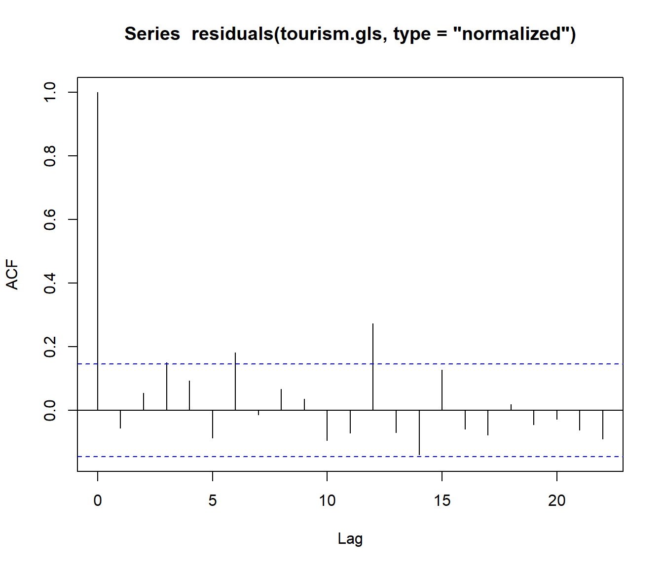
34.14 Comments on the Analysis
The estimated value of AR1 correlation parameter is \(\hat \phi = 0.393\).
Comparison of the output from
summary(tourism.gls)with the corresponding output from the earlier analysis (assuming independent errors) shows that the standard errors are usually larger here, particularly for the intercept and the coefficient ofTime:The only remaining question is, was the use of
gls()successful?We can get the normalized residuals (i.e. ‘decorrelated’ residuals) with