Lecture 29 Time Models with Independent Errors

29.1 Independent vs non-independent errors

Assumption A2 of linear regression \[ y_i = \beta_0 + \beta_1 x_{i1} + \beta_2 x_{2i} + ... \beta_p x_{pi} + \varepsilon_i\]

is that the errors \(\varepsilon_i\) are independent. That is, there is no carry-over of information from one data row \(i\) to another, apart from what is expressed through differences in the covariates (or factors, if relevant).

In the final topics of this course we will consider how to detect whether this assumption is broken, and how to model data with correlated errors \(cor(\varepsilon_{i-1},\varepsilon_i) \ne 0\).

For the moment we suppose the independence assumption A2 remains correct, and consider some simple ways of handling data that have a regular periodic component, such as patterns that depend on seasons of the year, or time of the day.

29.2 Indicator Variables for Seasonality

Often time series show some form of seasonal variation. One way to handle this in a regression equation is to use indicator variables which pick out the most obvious seasonal influences (e.g. summer/ winter, or the Christmas effect on retail figures. )

We consider data on Ski equipment sales versus PDI (personal disposable income). In the following data, both Ski Sales and PDI increased as time went by, but there appears to be a seasonal aspect to sales (which makes sense).

Download SkiSales.csv

## SkiSales = read.csv("SkiSales.csv", header = TRUE)
SkiSales |>
    head() |>
    kable()

Year	Quarter	Sales	PDI	Time
1964	1	37.0	109	1964.00
1964	2	33.5	115	1964.25
1964	3	30.8	113	1964.50
1964	4	37.9	116	1964.75
1965	1	37.4	118	1965.00
1965	2	31.6	120	1965.25

SkiSales |>
    mutate(Quarter = as.factor(Quarter)) |>
    ggplot(aes(y = Sales, x = PDI)) + geom_point(aes(pch = Quarter, col = Quarter))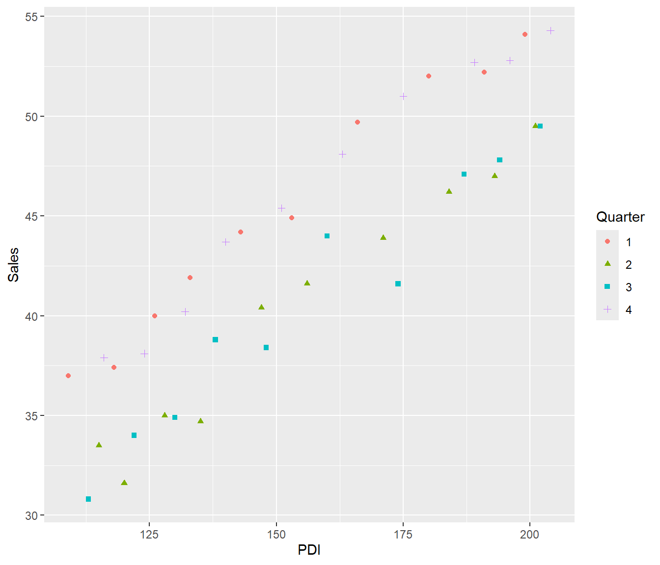

unlabelled

SkiSales.lm1 = lm(Sales ~ PDI, data = SkiSales)
Residuals = SkiSales.lm1$residuals
SkiSales |>
    mutate(Quarter = as.factor(Quarter)) |>
    ggplot(aes(x = PDI, y = Residuals)) + geom_point(aes(pch = Quarter, col = Quarter)) +
    geom_abline(h = 0)

Warning in geom_abline(h = 0): Ignoring unknown parameters: `h`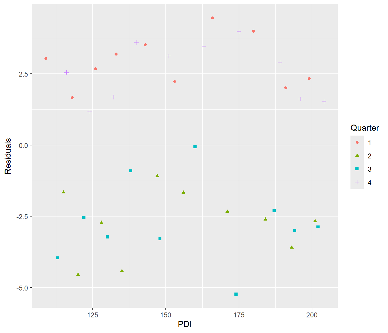

unlabelled

The residual plot shows that residuals tended to be positive in the first and fourth quarter of the year (plotted using o,x) and negative in second and third quarter (plotted using triangle,+). It therefore seems reasonable to create an indicator variable for winter (first and fourth quarter).

SkiSales |>
    mutate(Winter = as.numeric((Quarter == 1) + (Quarter == 4))) -> SkiSales
SkiSales.lm2 = lm(Sales ~ PDI + Winter, data = SkiSales)
summary(SkiSales.lm2)


Call:
lm(formula = Sales ~ PDI + Winter, data = SkiSales)

Residuals:
     Min       1Q   Median       3Q      Max 
-2.51118 -0.78640  0.02632  0.72842  2.67040 

Coefficients:
            Estimate Std. Error t value Pr(>|t|)    
(Intercept) 9.540202   0.974825   9.787 8.23e-12 ***
PDI         0.198684   0.006036  32.915  < 2e-16 ***
Winter      5.464342   0.359682  15.192  < 2e-16 ***
---
Signif. codes:  0 '***' 0.001 '**' 0.01 '*' 0.05 '.' 0.1 ' ' 1

Residual standard error: 1.137 on 37 degrees of freedom
Multiple R-squared:  0.9724,    Adjusted R-squared:  0.971 
F-statistic: 652.9 on 2 and 37 DF,  p-value: < 2.2e-16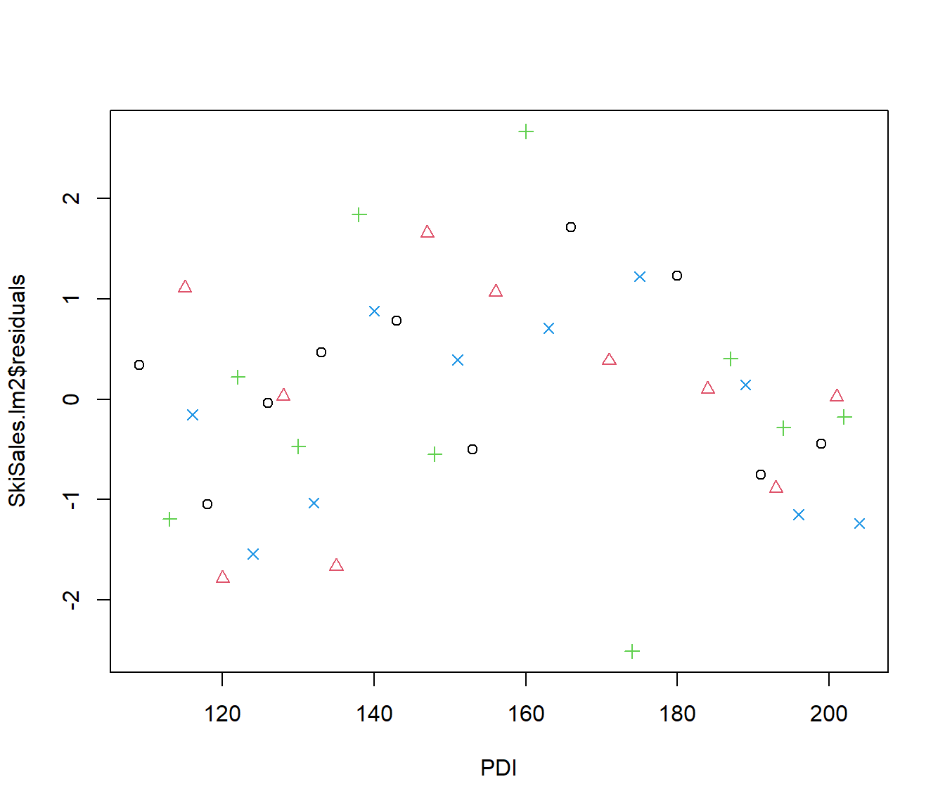

plot(SkiSales.lm2$residuals ~ PDI, pch = Quarter, col = Quarter, data = SkiSales)

unlabelled

The regression shows ski sales are significantly higher in winter, as expected, and the residuals do not show any particular pattern with Quarter.

However, for completeness, we will just check whether there is any tendency for ski sales to be higher or lower in the first half of winter (Christmas??) or summer.

SkiSales |>
    mutate(Q4 = as.numeric(Quarter == 4), Q2 = as.numeric(Quarter == 2)) -> SkiSales
SkiSales.lm3 = lm(Sales ~ PDI + Winter + Q4 + Q2, data = SkiSales)
summary(SkiSales.lm3)


Call:
lm(formula = Sales ~ PDI + Winter + Q4 + Q2, data = SkiSales)

Residuals:
     Min       1Q   Median       3Q      Max 
-2.51356 -0.86028  0.03654  0.67965  2.67306 

Coefficients:
             Estimate Std. Error t value Pr(>|t|)    
(Intercept)  9.479913   1.037830   9.134 8.58e-11 ***
PDI          0.199044   0.006190  32.155  < 2e-16 ***
Winter       5.645220   0.520508  10.846 9.72e-13 ***
Q4          -0.353116   0.521495  -0.677    0.503    
Q2           0.008279   0.519706   0.016    0.987    
---
Signif. codes:  0 '***' 0.001 '**' 0.01 '*' 0.05 '.' 0.1 ' ' 1

Residual standard error: 1.162 on 35 degrees of freedom
Multiple R-squared:  0.9728,    Adjusted R-squared:  0.9697 
F-statistic:   313 on 4 and 35 DF,  p-value: < 2.2e-16

anova(SkiSales.lm2, SkiSales.lm3)

Analysis of Variance Table

Model 1: Sales ~ PDI + Winter
Model 2: Sales ~ PDI + Winter + Q4 + Q2
  Res.Df    RSS Df Sum of Sq      F Pr(>F)
1     37 47.864                           
2     35 47.245  2   0.61919 0.2294 0.7962

We can conclude that a simple winter indicator is sufficient to express the effect of season on sales.

29.3 Effect of month

We consider some data on a householder’s monthly electricity bill from May 1994 to May 1998. During this period the householder sometimes let paying guests rent part of the house, and we may expect the electricity bill was higher at those times. The householder’s problem was to estimate the extra cost, so it could be legitimately claimed as a business expense for tax purposes.

One might expect the electricity bill to be higher in winter months, and in later years because of price rises, and also for periods when there were paying guests renting part of the house. It was also supposed that there might be an effect for the number of days included in the bill, and for whether the electricity bill was an estimate or the meter had actually been read.

The focus for us is how to adjust the analysis for the effect of season (month) on the bill. To examine this, we consider the residuals of Bill after adjusting for the non-weather-related variables.

Download Electricity.csv

## Electricity = read.csv("Electricity.csv", header = TRUE)
Electricity |>
    head() |>
    kable()

Bill	Days	Estimate	Guestwks	Month	Monthlab	Time	Year
70.18	29	0	0	5	M	5	94
79.05	30	1	0	6	J	6	94
78.60	27	0	0	7	J	7	94
81.45	29	1	0	8	A	8	94
174.25	28	0	4	9	S	9	94
115.20	28	1	0	10	O	10	94

Electricity.lm1 = lm(Bill ~ Days + Estimate + Guestwks + Time, data = Electricity)
resids = Electricity.lm1$residuals
plot(resids ~ Time, data = Electricity)
lines(resids ~ Time, lty = 1, col = 4, data = Electricity)
abline(h = 0, lty = 2)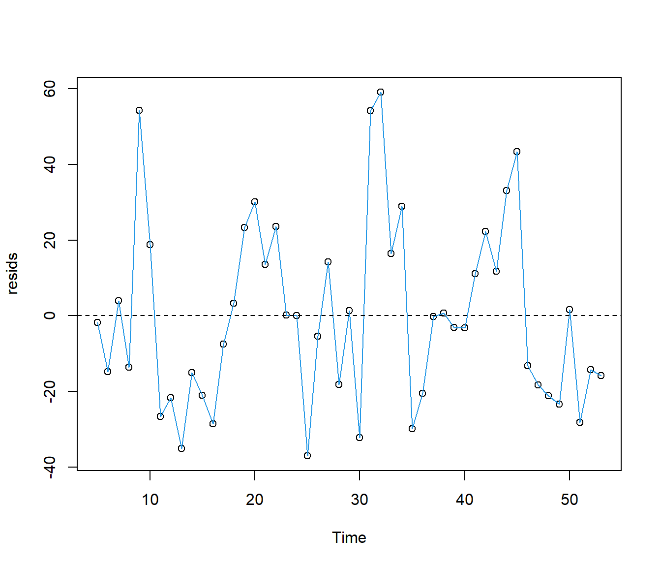

unlabelled

Although the effect of season is not clear, there are portions of the graph with several positive residuals in sequence, and several negative residuals. Time starts here at month=5 (May).

29.3.1 Indicator variables

One way of modelling seasonality would be to estimate an effect for each Month. The dataset here is really too short for such an approach, but we can try it for purposes of illustration.

Electricity.lm2 = lm(resids ~ factor(Month), data = Electricity)
summary(Electricity.lm2)


Call:
lm(formula = resids ~ factor(Month), data = Electricity)

Residuals:
    Min      1Q  Median      3Q     Max 
-40.822 -11.236   0.350   9.064  31.986 

Coefficients:
                Estimate Std. Error t value Pr(>|t|)    
(Intercept)      -23.929      8.953  -2.673 0.011125 *  
factor(Month)2    19.410     12.661   1.533 0.133785    
factor(Month)3    14.437     12.661   1.140 0.261517    
factor(Month)4     7.877     12.661   0.622 0.537669    
factor(Month)5    21.401     12.012   1.782 0.083015 .  
factor(Month)6    18.597     12.661   1.469 0.150341    
factor(Month)7    47.215     12.661   3.729 0.000642 ***
factor(Month)8    51.110     12.661   4.037 0.000262 ***
factor(Month)9    55.853     12.661   4.411 8.54e-05 ***
factor(Month)10   38.446     12.661   3.036 0.004368 ** 
factor(Month)11    5.300     12.661   0.419 0.677957    
factor(Month)12    8.133     12.661   0.642 0.524586    
---
Signif. codes:  0 '***' 0.001 '**' 0.01 '*' 0.05 '.' 0.1 ' ' 1

Residual standard error: 17.91 on 37 degrees of freedom
Multiple R-squared:  0.5794,    Adjusted R-squared:  0.4543 
F-statistic: 4.633 on 11 and 37 DF,  p-value: 0.0002005

We see from the F test that the mean(resids) varies significantly with Month.
F-statistic: 4.633 on 11 and 37 DF, p-value: 0.0002

The t-tests indicate that, compared to the baseline month January, the resids are unusually high in July through to October. This makes sense because more electricity would be used for lighting and heating during winter months.

Usually, however, we would like a more parsimonious model. So we consider one next.

29.4 Sinusoidal models

It would seem reasonable to model electricity use by temperature, and temperature by a simple Sine curve, with peak in winter and lowest electricity use in summer. Perhaps an initial guess is to set the ‘0’ for the sine curve to April since the power bill in that month includes the autumn equinox when temperatures should be ‘average’.

We can compute variables

SineTime=sin( (Time-4)\(\times 2\times\) 3.1415927 /12) , and

CosTime=cos( (Time-4)\(\times 2\times\) 3.1415927 /12).

The rationale for also calculating a Cosine curve is that sometimes we don’t know for sure where the ‘0’ should be. If we include a Cosine curve in the model, its effect is to allow the ‘0’ to shift earlier or later.

How it works: suppose we want to fit a curve of the form \(A\sin( x+\phi)\) where \(A\) is an amplitude and \(\phi\) is an unknown shift parameter. Then trigonometry tells us that \[A.\sin(x+\phi) =A\sin(x)\cos(\phi) + A\cos(x)\sin(\phi) \\ = A_1 \sin(x) + A_2\cos(x) \]

So a regression of \(Y\) on the two columns with numbers \(\sin(x)\) and \(\cos(x)\) will automatically calculate the slope parameters \(A_1\) and \(A_2\) and their relative size will automatically determine the optional choice of starting point \(\phi\). Easy as!

If we find out later the extra cos() term is not needed, then we can stick with our guess of April.

Electricity |>
    mutate(SinTime = sin((Time - 4) * 2 * 3.1415927/12), CosTime = cos((Time - 4) *
        2 * 3.1415927/12)) -> Electricity
Electricity.lm3 = lm(resids ~ SinTime + CosTime, data = Electricity)
summary(Electricity.lm3)


Call:
lm(formula = resids ~ SinTime + CosTime, data = Electricity)

Residuals:
    Min      1Q  Median      3Q     Max 
-43.135 -10.729  -2.141  11.561  37.675 

Coefficients:
              Estimate Std. Error t value Pr(>|t|)    
(Intercept)  -0.003126   2.756424  -0.001  0.99910    
SinTime      18.692199   3.917615   4.771 1.89e-05 ***
CosTime     -10.615098   3.878633  -2.737  0.00879 ** 
---
Signif. codes:  0 '***' 0.001 '**' 0.01 '*' 0.05 '.' 0.1 ' ' 1

Residual standard error: 19.29 on 46 degrees of freedom
Multiple R-squared:  0.3932,    Adjusted R-squared:  0.3669 
F-statistic: 14.91 on 2 and 46 DF,  p-value: 1.022e-05

The regression shows that the coefficient of CosTime is definitely non-zero. If it had been zero then this would mean \(\sin(\phi)=0\) and hence \(\phi=0\) or in other words that there was no need for any further adjustment from my guess of April as the “average” month.

Since the CosTime is highly significant it looks as if my guess was wrong. Let’s plot the fitted values on the same graph as my working ‘response’ variable.The plot below shows that the fitted values equal zero close to the first data point, at Time =5.

plot(resids ~ Time, data = Electricity)
lines(resids ~ Time, lty = 1, col = 4, data = Electricity)
lines(Electricity.lm3$fitted.values ~ Time, lty = 2, col = 2, lwd = 2, data = Electricity)
abline(h = 0, lty = 2)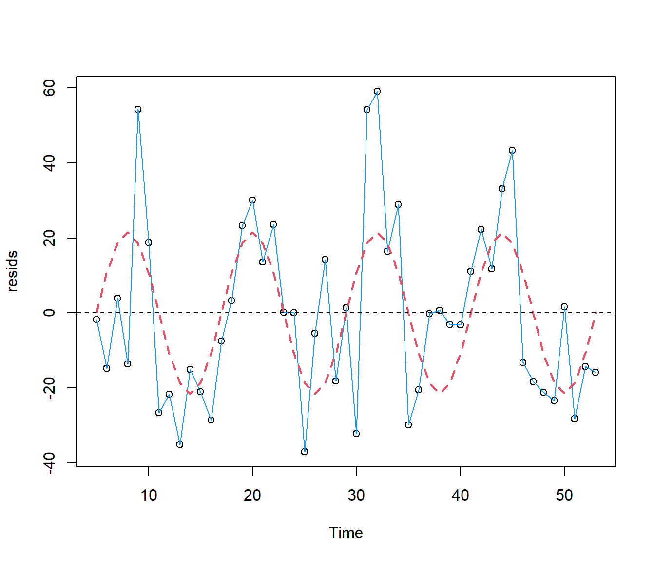

unlabelled

So we will try with 5 as the adjustment. The working below shows success.

Electricity |>
    mutate(SinTime = sin((Time - 5) * 2 * 3.1415927/12), CosTime = cos((Time - 5) *
        2 * 3.1415927/12)) -> Electricity
Electricity.lm4 = lm(resids ~ SinTime + CosTime, data = Electricity)
summary(Electricity.lm4)


Call:
lm(formula = resids ~ SinTime + CosTime, data = Electricity)

Residuals:
    Min      1Q  Median      3Q     Max 
-43.135 -10.729  -2.141  11.561  37.675 

Coefficients:
             Estimate Std. Error t value Pr(>|t|)    
(Intercept) -0.003126   2.756424  -0.001    0.999    
SinTime     21.495468   3.936961   5.460 1.85e-06 ***
CosTime      0.153155   3.858994   0.040    0.969    
---
Signif. codes:  0 '***' 0.001 '**' 0.01 '*' 0.05 '.' 0.1 ' ' 1

Residual standard error: 19.29 on 46 degrees of freedom
Multiple R-squared:  0.3932,    Adjusted R-squared:  0.3669 
F-statistic: 14.91 on 2 and 46 DF,  p-value: 1.022e-05

29.4.1 Adding more sin and cos terms

Now considering again the plot, I am not convinced that the relationship between resids and month is a simple sine curve. In particular resids rise more steeply in winter.

The next step is to add a component with double the period of the sin curve, i.e.

Sin2Time=sin( (Time-5)\(\times 4\times\) 3.1415927 /12) , and

Cos2Time=cos( (Time-5)\(\times 4\times\) 3.1415927 /12).

Adding terms in this way gives a more flexible set of shapes.

Electricity |>
    mutate(Sin2Time = sin((Time - 5) * 4 * 3.1415927/12), Cos2Time = cos((Time -
        5) * 4 * 3.1415927/12)) -> Electricity
Electricity.lm5 = lm(resids ~ SinTime + CosTime + Sin2Time + Cos2Time, data = Electricity)
summary(Electricity.lm5)


Call:
lm(formula = resids ~ SinTime + CosTime + Sin2Time + Cos2Time, 
    data = Electricity)

Residuals:
    Min      1Q  Median      3Q     Max 
-46.043 -13.531   0.651  11.336  34.987 

Coefficients:
            Estimate Std. Error t value Pr(>|t|)    
(Intercept)   0.2067     2.4900   0.083  0.93423    
SinTime      21.4955     3.5550   6.046 2.88e-07 ***
CosTime       0.5727     3.4873   0.164  0.87030    
Sin2Time     -6.1586     3.5550  -1.732  0.09022 .  
Cos2Time    -10.6995     3.4873  -3.068  0.00368 ** 
---
Signif. codes:  0 '***' 0.001 '**' 0.01 '*' 0.05 '.' 0.1 ' ' 1

Residual standard error: 17.42 on 44 degrees of freedom
Multiple R-squared:  0.5268,    Adjusted R-squared:  0.4837 
F-statistic: 12.24 on 4 and 44 DF,  p-value: 8.949e-07

anova(Electricity.lm4, Electricity.lm5)

Analysis of Variance Table

Model 1: resids ~ SinTime + CosTime
Model 2: resids ~ SinTime + CosTime + Sin2Time + Cos2Time
  Res.Df   RSS Df Sum of Sq      F   Pr(>F)   
1     46 17112                                
2     44 13346  2    3765.5 6.2072 0.004221 **
---
Signif. codes:  0 '***' 0.001 '**' 0.01 '*' 0.05 '.' 0.1 ' ' 1

plot(resids ~ Time, data = Electricity)
lines(resids ~ Time, lty = 1, col = 4, data = Electricity)
lines(Electricity.lm5$fitted.values ~ Time, lty = 2, col = 2, lwd = 2, data = Electricity)
abline(h = 0, lty = 2)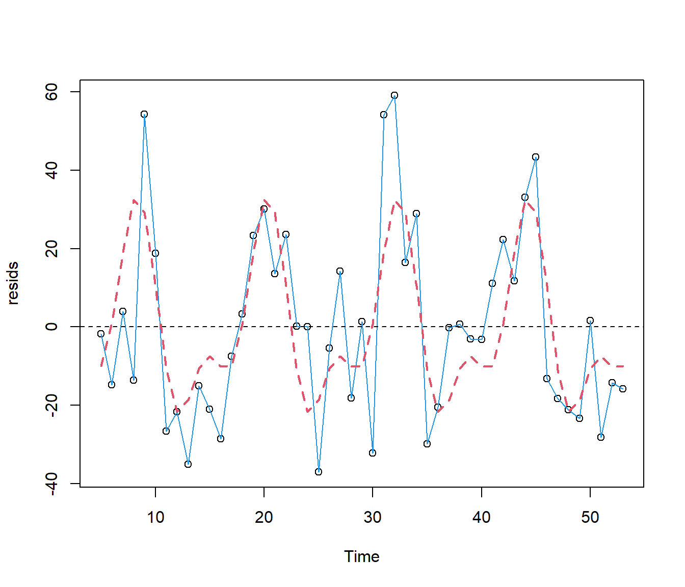

unlabelled

The regression output indicates that the extra sinusoidal terms have improved the fit significantly.

The graph suggests: first, that the peak in power costs in winter is steeper than previously shown, with estimated maximum in August; estimated minimum power use is in December; and there was a fairly flat period of electricity use for the four months between February and May inclusive.

(The graph actually shows a tiny peak in March but it is not clear whether this is real or an “artifact” of the model i.e. something forced by the fact we are fitting the data using simple wavy curves and so one is going to get wiggles whether real or not.)

The only way to check would be to add in even more terms such as sines and cosines with 3 times the frequency. However we do not have a lot of data so we will stop here.

29.4.2 Putting it together

Finally one should put all the variables together into the same model:

Electricity.lm6 = lm(Bill ~ Days + Estimate + Guestwks + Time + SinTime + CosTime +
    Sin2Time + Cos2Time, data = Electricity)
summary(Electricity.lm6)


Call:
lm(formula = Bill ~ Days + Estimate + Guestwks + Time + SinTime + 
    CosTime + Sin2Time + Cos2Time, data = Electricity)

Residuals:
    Min      1Q  Median      3Q     Max 
-37.718  -9.495  -0.918   9.350  34.942 

Coefficients:
            Estimate Std. Error t value Pr(>|t|)    
(Intercept)  24.2994    35.3845   0.687   0.4962    
Days          1.6721     1.2801   1.306   0.1989    
Estimate     10.6697     7.0672   1.510   0.1390    
Guestwks     11.0988     1.5241   7.282 7.62e-09 ***
Time          0.1432     0.1984   0.722   0.4745    
SinTime      27.0035     4.0213   6.715 4.68e-08 ***
CosTime      -1.5594     3.6114  -0.432   0.6682    
Sin2Time     -6.1630     3.4560  -1.783   0.0821 .  
Cos2Time     -7.5589     3.6172  -2.090   0.0430 *  
---
Signif. codes:  0 '***' 0.001 '**' 0.01 '*' 0.05 '.' 0.1 ' ' 1

Residual standard error: 16.84 on 40 degrees of freedom
Multiple R-squared:  0.7882,    Adjusted R-squared:  0.7458 
F-statistic:  18.6 on 8 and 40 DF,  p-value: 2.985e-11

plot(Bill ~ Time, data = Electricity)
lines(Bill ~ Time, lty = 1, col = 4, data = Electricity)
lines(Electricity.lm6$fitted.values ~ Time, lty = 2, col = 2, lwd = 2, data = Electricity)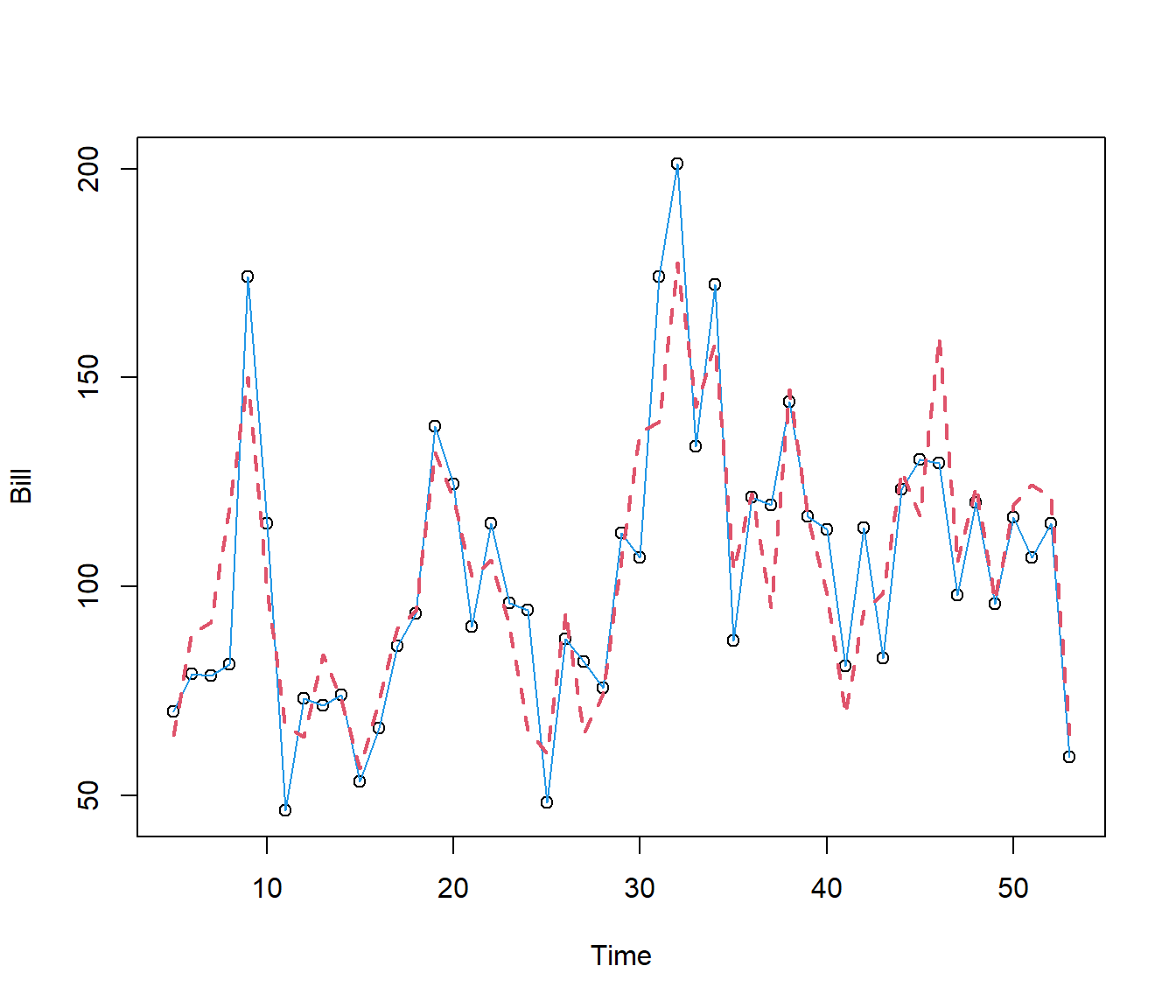

unlabelled

The model is not perfect, but is now picking up many of the features of the data.