Lecture 17 Models using orthogonal polynomials
We have seen that p-values for coefficients in a polynomial regression model will change depending upon what terms are included in the model.
This can be explained in terms of correlations between parameter estimates, described by their covariance matrix.
In this lecture we will discuss the construction of orthogonal polynomials, whose regression coefficients are uncorrelated.
17.1 Covariance Matrix for Parameter Estimates
We can explore the dependencies between estimates of individual regression coefficients using two matrices.
First, the covariance matrix for the regression parameter estimates which is given by \[\mbox{Var} \left( \hat{\boldsymbol{\beta}} \right) = \left ( \begin{array}{cccc} \mbox{Var} \left( \hat{\beta_0} \right) & \mbox{Cov} \left(\hat{\beta_0}, \hat{\beta_1}\right) & \ldots & \mbox{Cov} \left(\hat{\beta_0}, \hat{\beta_p} \right) \\ \mbox{Cov} \left(\hat{\beta_1}, \hat{\beta_0} \right) & \mbox{Var} \left( \hat{\beta_1} \right) & \ldots & \mbox{Cov} \left(\hat{\beta_1}, \hat{\beta_p} \right) \\ \vdots & \vdots & \ddots & \vdots \\ \mbox{Cov} \left(\hat{\beta_p}, \hat{\beta_0} \right) & \mbox{Cov} \left(\hat{\beta_p}, \hat{\beta_1} \right) & \ldots & \mbox{Var} \left(\hat{\beta_p} \right) \end{array} \right ) = \sigma^2 (X^T X)^{-1}\]
Where \(X\) is the design matrix and \(\sigma^2\) is the estimated standard error of the residuals.
17.2 Correlation Matrix for Parameter Estimates
From this, we can compute the second useful matrix: \[\mbox{Corr}\left( \hat{\boldsymbol{\beta}}\right) = \left ( \begin{array}{cccc} 1 & \mbox{Corr} \left(\hat{\beta_0}, \hat{\beta_1} \right) & \ldots & \mbox{Corr} \left(\hat{\beta_0}, \hat{\beta_p} \right) \\ \mbox{Corr} \left(\hat{\beta_1}, \hat{\beta_0} \right) & 1 & \ldots & \mbox{Corr} \left(\hat{\beta_1}, \hat{\beta_p} \right) \\ \vdots & \vdots & \ddots & \vdots \\ \mbox{Corr} \left(\hat{\beta_p}, \hat{\beta_0} \right) & \mbox{Corr} \left(\hat{\beta_p}, \hat{\beta_1} \right) & \ldots & 1 \end{array} \right )\]
following the definition of the correlation: \[cor(X, Y) = \frac{cov(X,Y)}{\sigma_X\sigma_Y}.\]
17.3 Crowds for the Brisbane Lions
This Data has the number of members and average crowds sizes for the Brisbane Lions AFL club from 1993 to 2003.
| Variables | Description |
|---|---|
| Year | Calendar year |
| Members | Number of Lions members |
| Crowd | Average home crowd size |
The aim of this Example is to regress Crowd on Year.

We first import, check and then plot the data.
'data.frame':   11 obs. of  3 variables:
 $ Year   : int  1993 1994 1995 1996 1997 1998 1999 2000 2001 2002 ...
 $ Members: int  5750 6158 6893 10267 16769 16108 16931 20295 18330 22288 ...
 $ Crowd  : int  11097 12437 10318 18672 19550 16669 22416 27283 28369 27565 ...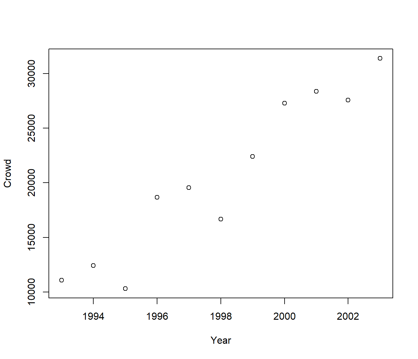
and then we can fit the model for the relationship of interest…
Call:
lm(formula = Crowd ~ Year, data = Lions)

Residuals:
    Min      1Q  Median      3Q     Max
-3856.1  -904.3   503.5  1355.8  2462.1

Coefficients:
              Estimate Std. Error t value Pr(>|t|)
(Intercept) -4270960.9   443882.4  -9.622 4.93e-06 ***
Year            2147.9      222.2   9.668 4.74e-06 ***
---
Signif. codes:  0 '***' 0.001 '**' 0.01 '*' 0.05 '.' 0.1 ' ' 1

Residual standard error: 2330 on 9 degrees of freedom
Multiple R-squared:  0.9122,    Adjusted R-squared:  0.9024
F-statistic: 93.47 on 1 and 9 DF,  p-value: 4.736e-06
As expected from the scatter plot, there is overwhelming evidence the Lion’s home crowds are increasing through time.
What does the intercept mean?
The covariance matrix for the estimates of the regression intercept and
slope, \(\hat{\beta_0}\) and \(\hat{\beta_1}\), can be extracted using R’s vcov()
command.
We can convert this covariance matrix to its corresponding correlation matrix using the cov2cor() command.
             (Intercept)         Year
(Intercept) 197031551082 -98614142.90
Year -98614143 49356.43 (Intercept) Year
(Intercept) 1.0000000 -0.9999987
Year -0.9999987 1.0000000Notice the dramatic negative correlation between \(\hat{\beta_0}\) and \(\hat{\beta_1}\).
This makes sense: if we change the slope of the regression line even a little bit, this will have a big impact on the value of the intercept (especially since the values of the explanatory variables are so far from 0).
17.4 Collinearity
This occurs because the rows of the design matrix (a
column of ones, and a column of the Year) are almost perfectly
collinear.
Collinearity means that one of the columns is (approximately) equal to a linear combination of the other columns.
In practice this means that it is difficult to distinguish between the effects of the variables in the model.
Hence the regression coefficients tend to be highly variable when collinearity occurs.
17.5 Introducing Orthogonal Polynomials
Let \(P_r(x_i)\) denote a polynomial of order \(r\) in \(x_i\), where \(i = 1, \ldots, n\); \[P_r(x_i) = a_0 + a_1x_i + a_2x_i^2 + \ldots + a_r x_i^r\]
The polynomials \(P_r\) and \(P_s\) are orthogonal if
\[\sum_{i=1}^n P_r(x_i) P_s(x_i) = 0~~~~~~(r \ne s)\]
We can fit a polynomial of order p to the data using orthogonal polynomials:
\[E[Y_i] = \alpha_0 + \alpha_1 P_1(x_i) + \alpha_2 P_2(x_i) + \ldots + \alpha_p P_p(x_i)\]
For example: \(E[Y_i] = 2+3x_i+4x_i^2\) can be re-expressed as
\[E[Y_i] = 1+3(\frac{1}{3}x_i+\frac{1}{3})+ 4(x_i^2+\frac{1}{2}x_i).\]
This will be completely equivalent to fitting \(E[Y_i] = \beta_0 + \beta_1 x_i + \beta_2 x_i^2 + \ldots + \beta_p x_i^p\) with the \(\beta\)’s being a simple transformation of the \(\alpha\)’s.
Fitting a polynomial regression using orthogonal polynomials means the resulting estimated regression coefficients are uncorrelated.
17.6 Constructing orthogonal polynomials for a simple regression
We can create a design matrix as follows:
\[X = \left [ \begin{array}{ll} 1 & x_1 - \bar x \\ 1 & x_2 - \bar x \\ \vdots & \vdots \\ 1 & x_n - \bar x \end{array} \right ]\]
Note: Columns of \(X\) are orthogonal because they can be expressed as two orthogonal polynomials.
Column 1 is \(P_0 = 1\).
Column 2 is \(P_1(x_i) = x_i - \bar{x}\).
We can show that \(\sum_{i=1}^n {P_0(x_i) P_1(x_i)} = \sum_{i=1}^n {(x_i - \bar{x})} = 0\).
When we have an orthogonal matrix X, wen have the following implications:
\(\rightarrow X^T X\) is a diagonal matrix
\(\rightarrow \sigma^2 (X^TX)^{-1}\) is also a diagonal matrix
\(\rightarrow\) parameter estimates based on a model with this design matrix will be uncorrelated.
17.7 Return to Brisbane Lions Example
We will define Yr to be a centred version of Year.
Lions$Yr <- Lions$Year - mean(Lions$Year)
Lions.lm2 <- lm(Crowd ~ Yr, data = Lions)
summary(Lions.lm2)
Call:
lm(formula = Crowd ~ Yr, data = Lions)

Residuals:
    Min      1Q  Median      3Q     Max
-3856.1  -904.3   503.5  1355.8  2462.1

Coefficients:
            Estimate Std. Error t value Pr(>|t|)
(Intercept)  20525.1      702.5  29.215 3.15e-10 ***
Yr            2147.9      222.2   9.668 4.74e-06 ***
---
Signif. codes:  0 '***' 0.001 '**' 0.01 '*' 0.05 '.' 0.1 ' ' 1

Residual standard error: 2330 on 9 degrees of freedom
Multiple R-squared:  0.9122,    Adjusted R-squared:  0.9024
F-statistic: 93.47 on 1 and 9 DF,  p-value: 4.736e-06
The models Lions.lm1 and Lions.lm2 have the same estimated slope parameters (as
expected).
The intercept parameter has changed, where \(\hat{\beta_0}\) now represents the mean value of the response when the covariate is at its sample mean value \(\bar{x}\).
            (Intercept)          Yr
(Intercept) 1.00000e+00 1.69369e-16
Yr          1.69369e-16 1.00000e+00
The regression parameter estimates now have zero correlation (R’s output is subject to slight numerical rounding errors).
Even if we change a little bit the slope of the regression line, it will still intersect with the x axis at the same intercept value.
17.8 Revisiting the FEV Data Example
Recall that in a previous Example we were fitting a polynomial
regression of FEV (a measure of lung function) on Age.
The estimated regression coefficients for this model are highly correlated.
## Fev <- read.csv(file = "fev.csv", header = TRUE)
Fev.lm6 <- lm(FEV ~ poly(Age, degree = 6, raw = TRUE), data = Fev)
cov2cor(vcov(Fev.lm6))
(Intercept)
(Intercept) 1.0000000
poly(Age, degree = 6, raw = TRUE)1 -0.9934543
poly(Age, degree = 6, raw = TRUE)2 0.9774233
poly(Age, degree = 6, raw = TRUE)3 -0.9558205
poly(Age, degree = 6, raw = TRUE)4 0.9313454
poly(Age, degree = 6, raw = TRUE)5 -0.9058334
poly(Age, degree = 6, raw = TRUE)6 0.8804847
poly(Age, degree = 6, raw = TRUE)1
(Intercept) -0.9934543
poly(Age, degree = 6, raw = TRUE)1 1.0000000
poly(Age, degree = 6, raw = TRUE)2 -0.9949850
poly(Age, degree = 6, raw = TRUE)3 0.9823511
poly(Age, degree = 6, raw = TRUE)4 -0.9650155
poly(Age, degree = 6, raw = TRUE)5 0.9450941
poly(Age, degree = 6, raw = TRUE)6 -0.9240672
poly(Age, degree = 6, raw = TRUE)2
(Intercept) 0.9774233
poly(Age, degree = 6, raw = TRUE)1 -0.9949850
poly(Age, degree = 6, raw = TRUE)2 1.0000000
poly(Age, degree = 6, raw = TRUE)3 -0.9960496
poly(Age, degree = 6, raw = TRUE)4 0.9859955
poly(Age, degree = 6, raw = TRUE)5 -0.9720506
poly(Age, degree = 6, raw = TRUE)6 0.9558551
poly(Age, degree = 6, raw = TRUE)3
(Intercept) -0.9558205
poly(Age, degree = 6, raw = TRUE)1 0.9823511
poly(Age, degree = 6, raw = TRUE)2 -0.9960496
poly(Age, degree = 6, raw = TRUE)3 1.0000000
poly(Age, degree = 6, raw = TRUE)4 -0.9968602
poly(Age, degree = 6, raw = TRUE)5 0.9888110
poly(Age, degree = 6, raw = TRUE)6 -0.9775523
poly(Age, degree = 6, raw = TRUE)4
(Intercept) 0.9313454
poly(Age, degree = 6, raw = TRUE)1 -0.9650155
poly(Age, degree = 6, raw = TRUE)2 0.9859955
poly(Age, degree = 6, raw = TRUE)3 -0.9968602
poly(Age, degree = 6, raw = TRUE)4 1.0000000
poly(Age, degree = 6, raw = TRUE)5 -0.9974864
poly(Age, degree = 6, raw = TRUE)6 0.9910050
poly(Age, degree = 6, raw = TRUE)5
(Intercept) -0.9058334
poly(Age, degree = 6, raw = TRUE)1 0.9450941
poly(Age, degree = 6, raw = TRUE)2 -0.9720506
poly(Age, degree = 6, raw = TRUE)3 0.9888110
poly(Age, degree = 6, raw = TRUE)4 -0.9974864
poly(Age, degree = 6, raw = TRUE)5 1.0000000
poly(Age, degree = 6, raw = TRUE)6 -0.9979756
poly(Age, degree = 6, raw = TRUE)6
(Intercept) 0.8804847
poly(Age, degree = 6, raw = TRUE)1 -0.9240672
poly(Age, degree = 6, raw = TRUE)2 0.9558551
poly(Age, degree = 6, raw = TRUE)3 -0.9775523
poly(Age, degree = 6, raw = TRUE)4 0.9910050
poly(Age, degree = 6, raw = TRUE)5 -0.9979756
poly(Age, degree = 6, raw = TRUE)6 1.0000000If we use the poly() function with the Age variable centred, we get…
Call:
lm(formula = FEV ~ poly(Age, degree = 6), data = Fev)

Residuals:
    Min      1Q  Median      3Q     Max
-1.2047 -0.2791  0.0186  0.2509  0.9210

Coefficients:
                       Estimate Std. Error t value Pr(>|t|)
(Intercept)             2.45117    0.02188 112.025  < 2e-16 ***
poly(Age, degree = 6)1  8.49647    0.39018  21.775  < 2e-16 ***
poly(Age, degree = 6)2 -3.14027    0.39018  -8.048 1.79e-14 ***
poly(Age, degree = 6)3 -0.35524    0.39018  -0.910    0.363
poly(Age, degree = 6)4  1.56999    0.39018   4.024 7.20e-05 ***
poly(Age, degree = 6)5  0.32921    0.39018   0.844    0.399
poly(Age, degree = 6)6 -0.28682    0.39018  -0.735    0.463
---
Signif. codes:  0 '***' 0.001 '**' 0.01 '*' 0.05 '.' 0.1 ' ' 1

Residual standard error: 0.3902 on 311 degrees of freedom
Multiple R-squared:  0.6418,    Adjusted R-squared:  0.6349
F-statistic: 92.87 on 6 and 311 DF, p-value: < 2.2e-16 (Intercept) poly(Age, degree = 6)1
(Intercept) 1 0
poly(Age, degree = 6)1 0 1
poly(Age, degree = 6)2 0 0
poly(Age, degree = 6)3 0 0
poly(Age, degree = 6)4 0 0
poly(Age, degree = 6)5 0 0
poly(Age, degree = 6)6 0 0
poly(Age, degree = 6)2 poly(Age, degree = 6)3
(Intercept) 0 0
poly(Age, degree = 6)1 0 0
poly(Age, degree = 6)2 1 0
poly(Age, degree = 6)3 0 1
poly(Age, degree = 6)4 0 0
poly(Age, degree = 6)5 0 0
poly(Age, degree = 6)6 0 0
poly(Age, degree = 6)4 poly(Age, degree = 6)5
(Intercept) 0 0
poly(Age, degree = 6)1 0 0
poly(Age, degree = 6)2 0 0
poly(Age, degree = 6)3 0 0
poly(Age, degree = 6)4 1 0
poly(Age, degree = 6)5 0 1
poly(Age, degree = 6)6 0 0
poly(Age, degree = 6)6
(Intercept) 0
poly(Age, degree = 6)1 0
poly(Age, degree = 6)2 0
poly(Age, degree = 6)3 0
poly(Age, degree = 6)4 0
poly(Age, degree = 6)5 0
poly(Age, degree = 6)6 117.9 Obtaining the design matrix
The model.matrix() command extracts the X matrix used in model fitting. It is quite large for the FEV data, so the following example compares the matrices used for the Lions example above.
   (Intercept) Year
1            1 1993
2            1 1994
3            1 1995
4            1 1996
5            1 1997
6            1 1998
7            1 1999
8            1 2000
9            1 2001
10           1 2002
11           1 2003
attr(,"assign")
[1] 0 1 (Intercept) Yr
1 1 -5
2 1 -4
3 1 -3
4 1 -2
5 1 -1
6 1 0
7 1 1
8 1 2
9 1 3
10 1 4
11 1 5
attr(,"assign")
[1] 0 1In this simple regression, it is relatively easy to see the manipulation that took effect. We will see another situation when the design matrix helps us understand the way our models are fitted in a lecture coming soon…
The re-scaling of a variable is not limited to polynomial regression situations. Re-scaling of a variable could prove worthwhile in any regression context when that variable has a relatively small range as compared to its distance from zero.
17.8.1 Comments
We have fitted a 6th order polynomial regression of
FEVonAgeusing orthogonal polynomials.The R function constructed the necessary polynomials in a manner that can be used as explanatory variables in a linear model.
Note that the
polyfunction will construct by default orthogonal polynomials. To get non-orthogonal polynomials we need to addraw = TRUEinside thepoly()function.The fitted 6th order model using orthogonal polynomials produces identical fits (and predictions) to the 6th order model constructed in the original case study using the raw polynomial values or the
I()function.We use the
round()command to remove rounding error in the output.You should see that you get an identity matrix in return. This tells you that the estimate regression coefficients for the model are uncorrelated.
As a result of the estimates not being correlated, we can interpret t-test statistics and p-values in the summary table independently.
That is, p-values will not change much when we remove terms from the model.
The summary table shows us straight away that we need a polynomial of 4th order to model
FEVas a function ofAge.