Lecture 35 Regression with Autoregressive Errors
35.1 Regression with Autoregressive Errors
In Lecture 34 we found that a regression can explain the mean quite well and still leave neighbouring residuals related. If this month’s response is above the fitted mean, next month’s deviation may also be positive. How can we account for that dependence when estimating the regression coefficients and their precision?
By the end of this lecture, students should be able to:
- Write down a regression model with AR(1) errors.
- Explain why autocorrelated errors distort ordinary standard errors.
- Fit a regression model with
gls()andcorAR1(). - Check whether normalised residuals look closer to white noise.
35.2 Main Worked Example: Tourism in Victoria
These data record monthly room nights occupied in hotels, motels, and guesthouses in Victoria from January 1980 to December 1994. We have 180 observations, one for each month.
tourism <- read_csv("../data/motel.csv", show_col_types = FALSE) |>
    mutate(Date = as.Date(Date), Time = round(time_length(Date - min(Date), unit = "month")),
        Month = factor(month(Date, label = TRUE), ordered = FALSE), Year = year(Date)) |>
    arrange(Date)

stopifnot(nrow(tourism) == 180, all(diff(tourism$Time) == 1))
Time counts months from the start of the series. Month lets expected room nights differ between January, February, and so on.
35.3 Tourism: Fit the Mean First
We allow a linear trend and a separate effect for each month:
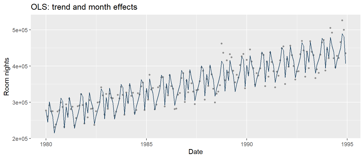
The fitted mean follows much of the growth and seasonal variation. Now check the deviations around it.
35.4 Tourism: What Remains Over Time?
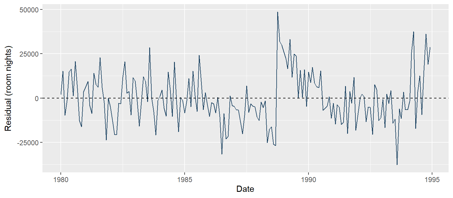
Follow the residuals in time order. Several consecutive months can sit on the same side of zero even after fitting trend and month effects. A seasonal pattern in the mean and dependence among the errors are different parts of the model.
35.5 Tourism: ACF Before GLS
acf(resid(tourism_lm), lag.max = 24, main = "OLS tourism residuals", xlab = "Lag (months)",
    ylim = c(-0.4, 1))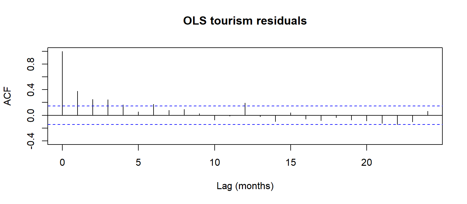
Lag 1 is one month; lag 12 is one year. The lag-1 correlation is about 0.377, with positive correlations at several nearby lags. An AR(1) error model is a reasonable first attempt to account for that persistence.
35.6 Why Ordinary Least Squares Is Not Enough
If the mean model is correctly specified and the errors average to zero given the predictors, correlated errors do not by themselves make the OLS coefficients biased.
The usual OLS standard errors still assume independent errors. When nearby deviations tend to move together, their contribution to precision differs from that calculation. Confidence intervals and tests based on it can therefore be unreliable.
We will keep the same trend and month predictors and change the model for the errors. The direction and size of the standard-error change depend on the predictors and the dependence pattern.
35.7 The AR(1) Error Model
A first-order autoregressive, or AR(1), error model is
\[\varepsilon_t = \phi\varepsilon_{t-1} + \eta_t.\]
The current error contains a contribution from the previous error, \(\phi\varepsilon_{t-1}\), plus a new disturbance, \(\eta_t\). We call \(\eta_t\) the innovation: the part that was not carried forward from the past.
We assume the innovations are independent of past errors and of one another, with mean zero and constant variance.
- If \(\phi>0\), nearby errors tend to move in the same direction.
- If \(\phi<0\), nearby errors tend to alternate.
- If \(\phi=0\), each error is just its new innovation.
35.8 AR(1): Put Numbers Into the Equation
Suppose \(\phi=0.4\) and last month’s error was 1,000 room nights. The contribution carried into this month is
\[\phi\varepsilon_{t-1}=0.4\times1{,}000=400.\]
If this month’s error is 500, the new disturbance must be
\[\eta_t=\varepsilon_t-\phi\varepsilon_{t-1}=500-400=100.\]
The model separates the 500 into 400 carried forward and 100 of new disturbance. Before observing this month’s innovation, its expected error would be 400. The realised error can differ because a new disturbance arrives.
These are illustrative errors. In real data we do not know the true errors, so we estimate the mean and work with residuals.
35.9 How Long Does the Dependence Last?
For a stationary AR(1) process, the lag-\(k\) error correlation is \(\phi^k\). With \(\phi=0.4\):
| Time gap | Correlation |
|---|---|
| One month | \(0.4\) |
| Two months | \(0.4^2=0.16\) |
| Three months | \(0.4^3=0.064\) |
The previous error carries information about the next one, but that information weakens across longer gaps.
We require \(|\phi|<1\) for a stationary AR(1) error process. Here stationary means the error process has a stable mean and variance, and correlations depend on the time gap. The response itself can still have trend and seasonality through its mean model.
35.10 Regression Model with AR(1) Errors
For the tourism data, our two model components are
\[\begin{aligned} Y_t &= \beta_0 + \beta_1\mathrm{Time}_t + \beta_2z_{t,2} + \cdots + \beta_{12}z_{t,12} + \varepsilon_t, \\ \varepsilon_t &= \phi\varepsilon_{t-1} + \eta_t. \end{aligned}\]
The \(z_{t,j}\) terms are the 11 month indicators, with January as the reference month.
The first equation describes expected room nights given time and month. The second describes how deviations from that expectation persist. Adding AR(1) errors does not add last month’s observed room nights as a predictor in the mean formula.
35.11 Why GLS Works: Compare Two Adjacent Times
To see the calculation with one predictor, write the regression at times \(t\) and \(t-1\):
\[\begin{aligned} y_t &= \beta_0 + \beta_1x_t + \varepsilon_t, \\ y_{t-1} &= \beta_0 + \beta_1x_{t-1} + \varepsilon_{t-1}. \end{aligned}\]
Multiply the second equation by \(\phi\). Subtracting it from the first leaves the error difference
\[\varepsilon_t-\phi\varepsilon_{t-1}=\eta_t.\]
Under the AR(1) model, this difference is the new innovation. We have removed the contribution carried forward from the previous error.
35.12 Why GLS Works: Transform the Whole Regression
Subtracting the two equations gives
\[y_t-\phi y_{t-1} =\beta_0(1-\phi)+\beta_1(x_t-\phi x_{t-1})+\eta_t.\]
- The response becomes \(y_t-\phi y_{t-1}\).
- The predictor becomes \(x_t-\phi x_{t-1}\).
- The intercept multiplier becomes \(1-\phi\).
We must transform the whole regression, including every predictor. Transforming only the response would describe a different mean model.
Generalised least squares (GLS) uses the error covariance structure to estimate the regression coefficients. This adjacent-time calculation explains its mechanism for AR(1); the software also handles the first observation and estimates the unknown \(\phi\).
35.13 Fitting the AR(1) Model in R
gls() from nlme takes the usual mean formula plus a correlation structure:
RoomNights ~ Time + Month specifies the mean. corAR1(form = ~ Time) specifies how errors are related according to their separation in time.
Time must be integer-valued and counts months here. Observations two months apart have modelled error correlation \(\phi^2\), rather than \(\phi\).
35.14 Tourism: Interpret the Estimated Dependence
| Gap (months) | Fitted error correlation |
|---|---|
| 1 | 0.393 |
| 2 | 0.154 |
| 3 | 0.061 |
We estimate \(\hat\phi\approx 0.393\). After allowing for trend and month effects, errors one month apart have an estimated correlation of about 0.39 under this model.
That estimate describes the modelled dependence. We still need to check whether the model accounts for the pattern in these data.
35.15 How Precisely Have We Estimated the Correlation?
\(\hat\phi\) is an estimate from 180 months of data, so it carries uncertainty of its own.
Approximate 95% confidence intervals

 Coefficients:
                  lower       est.      upper
(Intercept) 266228.1202 275492.204 284756.287
Time           999.3307   1062.250   1125.169
MonthFeb    -39495.9823 -31194.086 -22892.190
MonthMar     13691.2693  23482.727  33274.185
MonthApr    -12487.0081  -2170.467   8146.074
MonthMay    -29933.5149 -19419.121  -8904.728
MonthJun    -76415.1029 -65827.114 -55239.126
MonthJul    -55130.5097 -44522.343 -33914.177
MonthAug    -40361.8121 -29768.745 -19175.677
MonthSept   -22565.9807 -12039.271  -1512.561
MonthOct     16051.4987  26393.955  36736.411
MonthNov      6623.9585  16471.666  26319.373
MonthDec    -67066.8155 -58631.939 -50197.063

 Correlation structure:
        lower     est.     upper
Phi 0.2419081 0.392721 0.5250065

 Residual standard error:
   lower     est.    upper
13041.25 14799.38 16794.53
The Phi row repeats our estimate and adds an approximate 95% interval for the error correlation. In Lab 13 you will read the same row for the Perth house-price data, where only 45 quarters are available and the interval is wider.
The lesson to carry forward: an estimate of \(\phi\) near zero does not by itself establish independence when the interval around it is wide.
35.16 Where Does the GLS Standard Error Come From?
Lecture 34 wrote down the variance OLS reports when independence fails. GLS uses the fitted error model instead:
\[\operatorname{Var}(\widehat{\boldsymbol\beta}_{\text{GLS}}) =(X^\top\widehat\Sigma^{-1}X)^{-1}.\]
\(\widehat\Sigma\) is the estimated error covariance matrix. For AR(1) errors it is assembled from \(\hat\phi\) and \(\hat\sigma\), because this model fixes \(\operatorname{Corr}(\varepsilon_s,\varepsilon_t)=\phi^{|s-t|}\). Here \(\hat\sigma\) is the innovation standard deviation, the scale of the new disturbances \(\eta_t\): summary(tourism_gls) reports it as the residual standard deviation, and the raw errors themselves have variance \(\sigma^2/(1-\phi^2)\).
Neither parameter is known in advance, so gls() estimates \(\phi\) and \(\sigma\) alongside the regression coefficients. When neighbouring errors carry overlapping information, \((X^\top\widehat\Sigma^{-1}X)^{-1}\) can give larger variances than the independent-errors formula, even with an almost unchanged mean fit. The comparison below is where that shows up.
35.17 Tourism: What Happens to the Trend and Its Precision?
| Model | Trend estimate | Standard error |
|---|---|---|
| OLS | 1058.8 | 21.2 |
| GLS with AR(1) | 1062.2 | 31.9 |
Holding month constant, expected room nights increase by about 1,062 for each additional month. The trend estimate barely changes between the two fits.
Its standard error increases by about 51%. A similar fitted mean can have a different precision calculation once we account for dependence. GLS can also change coefficient estimates; neither the direction nor the size of these changes is universal.
Selection inherits this change. Comparing models by AIC ranks them using the fitted error model, and judging a term by its t-statistic reads the standard errors shown here, so an error model can change which terms look worth keeping. Any such comparison between models with different mean formulas should be made with method = "ML" in gls(), since the default REML likelihood is intended for models sharing a mean structure.
35.18 Which GLS Residuals Should We Check?
The raw GLS residual is still observed minus fitted:
\[e_t=y_t-\widehat\mu_t.\]
Our model allows these deviations to be correlated. We should therefore expect raw residuals to retain some of that correlation, even when the error model is reasonable.
Normalised residuals account for the fitted correlation and rescale the residuals. For adjacent times in this AR(1) example, the calculation is based on \(e_t-\hat\phi e_{t-1}\), followed by scaling. We check these for remaining dependence.
The name normalised describes that transformation. It does not mean the residual distribution has been made normal. See the nlme residual documentation.
35.19 Tourism: Raw and Normalised Residuals
tourism_raw <- residuals(tourism_gls, type = "response")
tourism_normalised <- residuals(tourism_gls, type = "normalized")| Residuals | Lag-1 correlation | Lag-12 correlation |
|---|---|---|
| OLS | 0.377 | 0.192 |
| GLS: raw | 0.378 | 0.193 |
| GLS: normalised | -0.057 | 0.272 |
The raw GLS residuals have much the same lag-1 correlation as the OLS residuals. After accounting for the fitted dependence, the normalised residuals have much less lag-1 correlation. The lag-12 value still needs attention.
35.20 Tourism: Residual Patterns Before and After GLS
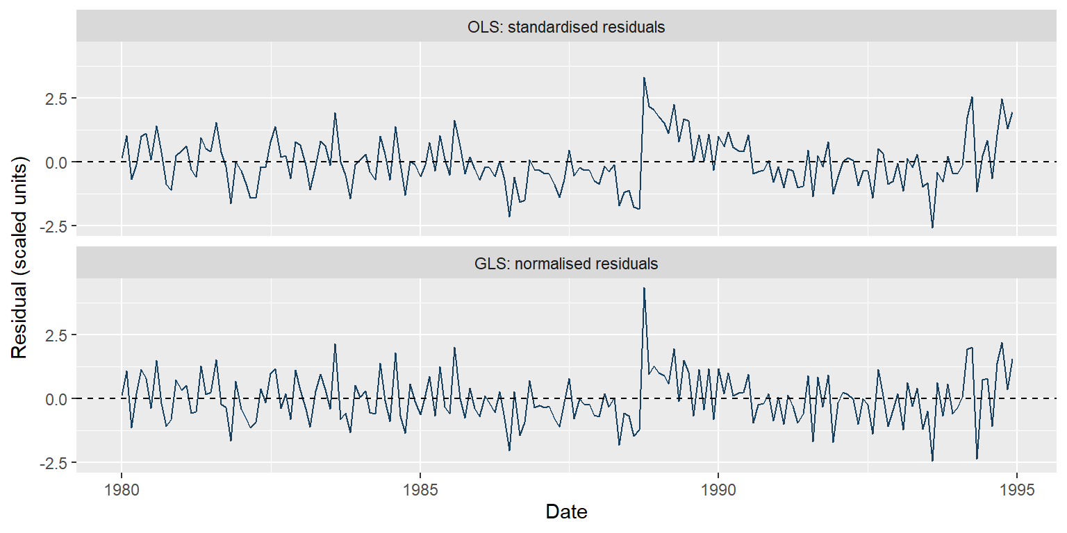
Both plots use the same months. The OLS residuals are divided by their estimated residual standard deviation to put them on a comparable scale. Look for persistence in the sequence, as well as large individual deviations.
35.21 Tourism: ACF Before and After GLS
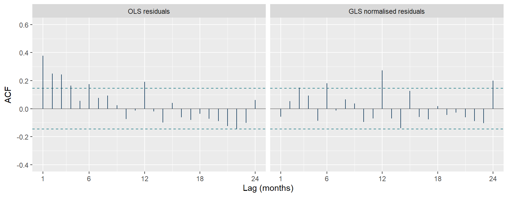
Lag 0 is omitted because it is always 1. The panels have identical axes. Lag 1 falls from 0.377 to -0.057, but lag 12 remains positive at 0.272.
The dashed lines are approximate pointwise white-noise reference limits. They guide inspection; they do not prove independence or form a simultaneous band across all lags.
35.22 Tourism: Repeat Ljung-Box Across One Year
The ACF shows where correlation remains. Ljung-Box combines the correlations across a chosen set of lags. Use lags 1 through 12 to include gaps of up to one year:
\[H_0:\rho_1=\cdots=\rho_{12}=0.\]
tourism_lb_ols <- Box.test(resid(tourism_lm), lag = 12, type = "Ljung-Box", fitdf = 0)
tourism_lb_gls <- Box.test(tourism_normalised, lag = 12, type = "Ljung-Box", fitdf = 1)
We chose 12 using the monthly time scale, rather than searching for a lag that gives a preferred P-value.
35.23 Tourism: Has the Dependence Been Accounted For?
| Residuals | Statistic Q | Reference df | Approximate P-value |
|---|---|---|---|
| OLS | 71.03 | 12 | < 1e-04 |
| GLS: normalised | 32.74 | 11 | 0.000579 |
The statistic is smaller after normalisation, and the lag-1 correlation is much reduced. The remaining small P-value and lag-12 ACF bar still give evidence of dependence across these lags.
35.24 Tourism: What Would We Investigate Next?
The month indicators already allow the average January mean to differ from the average February mean. They do not necessarily account for changing seasonal effects or dependence between deviations one year apart.
I would check whether the trend or seasonal mean is missing structure, then consider whether the errors need a richer model for seasonal dependence. The lag-12 bar identifies a time gap to investigate; it does not identify the correct replacement model.
Correlation magnitude tells us how large a particular sample relationship is. A P-value measures evidence against a reference hypothesis. A larger P-value, or a smaller Ljung-Box statistic, would not establish that all dependence had been resolved.
35.25 Work Through the AR(1) Calculation
Suppose \(\phi=0.6\), the previous error is \(-200\), and the current error is \(-50\). What is the innovation?
. . .
The contribution carried forward is \(0.6\times(-200)=-120\). Therefore
\[\eta_t=-50-(-120)=70.\]
The new disturbance is positive even though the current error is negative. It partly offsets the negative contribution from the past.
35.26 Which Residuals Answer Our Diagnostic Question?
After fitting AR(1) errors, the raw GLS residuals still have positive lag-1 correlation. Does that alone show the model failed?
. . .
No. The model allows raw deviations from the fitted mean to be correlated. We inspect normalised residuals to ask whether dependence remains after accounting for the fitted error structure.
A large estimated \(\phi\) and a small normalised lag-1 correlation can occur together: the model has estimated substantial dependence and accounted for much of it.
35.27 Interpret the Before-and-After ACF
Lag-1 correlation is close to zero after normalisation, but lag-12 correlation remains large. What conclusion can we draw?
. . .
AR(1) has accounted for much of the neighbouring-month dependence. It has left a pattern at a one-year gap, so we should investigate the mean and the error model further.
Checking only lag 1 would miss that remaining pattern. We need the time plot, the wider ACF and a joint diagnostic, rather than a single numerical verdict.
35.28 A Short Comparison: Seoul Bike with AR(1) Errors
Return to the daily Seoul bike model from Lectures 32/33. Its mean includes the time trend, two Fourier pairs and weather predictors. We now fit both OLS and GLS to all functioning days.
seoul_lm <- lm(rented_bike_count ~ day_index + S1 + C1 + S2 + C2 + mean_temperature +
total_rainfall + total_solar_radiation, data = seoul_daily)S1, C1, S2 and C2 are the same annual seasonal terms used earlier. The mean formula is held constant for the comparison.
35.29 Seoul: Fit AR(1) Using Actual Day Distances
seoul_gls <- gls(rented_bike_count ~ day_index + S1 + C1 + S2 + C2 + mean_temperature +
    total_rainfall + total_solar_radiation, correlation = corAR1(form = ~day_index),
    data = seoul_daily)
Both models use all 352 functioning days. We retain the original day_index after removing the 13 outage days. A gap of three days therefore has modelled error correlation \(\phi^3\), rather than being treated as one step.
Here \(\hat\phi\approx 0.503\). The next question is whether the normalised residuals show less dependence.
35.30 Seoul: Compare Estimates and Standard Errors
| Model | Trend estimate | Standard error |
|---|---|---|
| OLS | 12.68 | 3.80 |
| GLS with AR(1) | 10.07 | 6.46 |
The day-index coefficient is the change in expected daily rentals per additional day, holding the seasonal and weather predictors constant. Its estimate changes from 12.68 to 10.07, while its standard error increases.
As in tourism, accounting for dependence changes the precision calculation. Here it also makes a more visible difference to the trend estimate.
35.31 Seoul: Make a Matched Diagnostic Comparison
An ordinary ACF assumes equally spaced observations. Use the uninterrupted period from 1 December 2017 to 10 April 2018 for both residual sequences:
seoul_run <- seoul_diagnostics |>
    filter(date >= as.Date("2017-12-01"), date <= as.Date("2018-04-10"))

stopifnot(nrow(seoul_run) == 131, all(diff(seoul_run$day_index) == 1), all(as.numeric(diff(seoul_run$date)) ==
    1))
Both models were fitted on 352 days; these plots examine their residuals on the same 131-day window. Lecture 34 refitted the mean model on that window. Its residuals therefore differ from the full-year OLS residuals compared here.
35.32 Seoul: ACF Before and After GLS
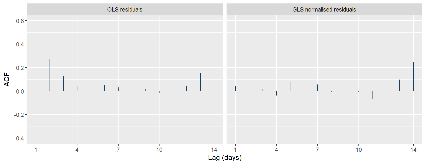
Lag-1 correlation falls from 0.549 to 0.042. There is much less neighbouring-day dependence in this window, although the lag-14 bar still stands out.
These plots do not establish adequacy across the whole year. We have not treated the gappy 352-row series as equally spaced, or applied a formal Ljung-Box test to this selected window.
35.33 What Would You Check After Fitting GLS?
Keep the mean and error questions separate. A plausible trend and seasonal mean can still leave dependence, and a fitted AR(1) parameter does not establish that the error model is adequate.
Inspect normalised residuals in time order, compare their ACF with the original residual ACF, and interpret a joint diagnostic where appropriate. Check longer gaps as well as lag 1.
For tourism, we have accounted for much of the short-term persistence, while seasonal dependence remains worth investigating. For Seoul, the matched window shows a substantial improvement, with conclusions limited to that period. In each case, the next modelling decision comes from what remains in the residuals.
35.34 Looking Forward
We stop at AR(1) errors: the simplest model we could write for dependence between neighbouring observations. The same move, choosing a structure for \(\Sigma\) and estimating it alongside the mean, is the working heart of several fields this course does not reach.
- ARIMA models: the standard forecasting toolkit. Differencing removes a trend before fitting, and autoregressive and moving-average terms let the errors carry longer memory than our single \(\phi\). Used for short-term forecasts of demand, energy and economic series, each issued with a prediction interval.
- GARCH models: for returns and other series where volatility itself is correlated. Today’s variance is written as a function of yesterday’s squared innovations, so calm stretches follow calm and wild follow wild. Banks and insurers build risk measures on it.
- Mixed models: for grouped data such as repeated measurements on the same patient, plot or school. Each group receives its own coefficient drawn from a shared distribution, which builds a block structure into \(\Sigma\). The workhorse of longitudinal and clinical studies.
- Gaussian processes: replace the fixed \(\phi^k\) decay with a covariance function of distance. The joint distribution of fitted values then gives prediction intervals that widen away from the data. This is kriging in geostatistics and the surrogate behind Bayesian optimisation in machine learning.
All four reuse the move we made today: model the covariance, estimate it with the mean, and let the residuals say whether more structure is needed.