Lecture 31 Splines and LOESS: Flexible Regression Curves
31.1 Splines and LOESS: Flexible Regression Curves
So far most of our mean models have imposed a fairly simple global shape. In this lecture we use the Seoul Bike Sharing data to deal with a different problem: the relationship between demand and weather is clearly nonlinear. We want the mean response to bend where the data support it without giving up the regression framework.
By the end of this lecture, students should be able to:
- Explain why a straight-line mean function can be too restrictive.
- Use LOESS to explore nonlinear structure.
- Explain how cubic splines use knots to let a regression curve change shape smoothly.
- Fit and interpret cubic and natural cubic splines.
- Explain how degrees of freedom control the flexibility of a cubic spline.
31.2 Running Example: Hourly Bike Demand
Download seoul_bike_hourly.csv
# A tibble: 8,760 × 16
   date       datetime            day_index  hour rented_bike_count temperature
   <date>     <dttm>                  <dbl> <dbl>             <dbl>       <dbl>
 1 2017-12-01 2017-12-01 00:00:00         1     0               254        -5.2
 2 2017-12-01 2017-12-01 01:00:00         1     1               204        -5.5
 3 2017-12-01 2017-12-01 02:00:00         1     2               173        -6
 4 2017-12-01 2017-12-01 03:00:00         1     3               107        -6.2
 5 2017-12-01 2017-12-01 04:00:00         1     4                78        -6
 6 2017-12-01 2017-12-01 05:00:00         1     5               100        -6.4
 7 2017-12-01 2017-12-01 06:00:00         1     6               181        -6.6
 8 2017-12-01 2017-12-01 07:00:00         1     7               460        -7.4
 9 2017-12-01 2017-12-01 08:00:00         1     8               930        -7.6
10 2017-12-01 2017-12-01 09:00:00         1     9               490        -6.5
# ℹ 8,750 more rows
# ℹ 10 more variables: humidity <dbl>, wind_speed <dbl>, visibility <dbl>,
#   dew_point_temperature <dbl>, solar_radiation <dbl>, rainfall <dbl>,
#   snowfall <dbl>, season <chr>, holiday <chr>, functioning_day <chr>
The core question for this lecture is:
How does hourly bike demand change with temperature?
31.2.1 Why Go Beyond Straight Lines?
A straight-line model can underfit. A highly flexible curve can overfit. Our aim is to describe the mean relationship without losing the regression framing.
seoul_hourly |>
    ggplot(aes(x = temperature, y = rented_bike_count)) + geom_point(alpha = 0.06) +
    labs(x = "Temperature (C)", y = "Hourly rented bike count", title = "Bike demand changes nonlinearly with temperature")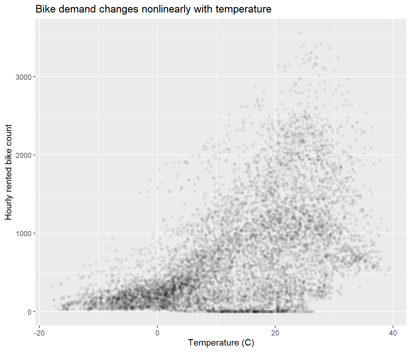
31.3 Example 1: LOESS
31.3.1 The LOESS Idea
LOESS fits a separate regression at each predictor value where we want an estimate. At a target value \(x_0\), R’s default LOESS fit uses a local quadratic working model for observations near \(x_0\):
\[Y_i = \beta_0(x_0) + \beta_1(x_0)(x_i-x_0) + \beta_2(x_0)(x_i-x_0)^2 + \varepsilon_i.\]
The coefficients depend on \(x_0\). We choose them to minimise the weighted sum of squares
\[\sum_{i=1}^n w_i(x_0)\left\{y_i-\beta_0(x_0)-\beta_1(x_0)(x_i-x_0)-\beta_2(x_0)(x_i-x_0)^2\right\}^2.\]
31.3.2 Local Weights
Observations close to \(x_0\) receive more weight, while observations outside its neighbourhood or span receive none. Because we have centred the predictor at \(x_0\), the fitted value there is \(\hat f(x_0)=\hat\beta_0(x_0)\). Repeat the calculation at other values of \(x_0\) and those fitted values form the curve. There is no single set of quadratic coefficients for the whole predictor range.
These are distance weights. In the previous lecture, we used weights to account for differences in precision; here the weights decide which observations matter for a local fit. For an observation inside the neighbourhood of \(x_0\), the usual tricube weight is
\[ w_i(x_0)=\left[1-\left(\frac{|x_i-x_0|}{d(x_0)}\right)^3\right]^3, \]
with weight zero outside the neighbourhood. Here \(d(x_0)\) is the distance to its edge. The nearest observations receive the largest weights.
The distinction between these distance weights and Lecture 30’s precision weights is span sets the proportion of X% ‘closest’ points. Therefore a span of 1 is all points in a neighbourhood around \(x_0\) and .25 is a quarter of the points closest to \(x_0\). Therefore, a small span gives a flexible curve that can follow random fluctuations. A larger span borrows from farther away, producing a smoother curve that may miss a sharp change in the mean.
The weight formula is not examinable;
31.4 LOESS: Span
31.4.1 Seoul Bike Data
We have already fitted polynomials and piecewise regression models. A polynomial uses one global curve, so changing its coefficients can alter the fit across the entire range. A piecewise model lets the shape change at selected predictor values. Here LOESS gives us another view of the relationship between temperature and bike demand before we commit to a particular regression formula.
seoul_hourly |>
    ggplot(aes(x = temperature, y = rented_bike_count)) + geom_point(alpha = 0.05) +
    geom_smooth(method = "loess", formula = y ~ x, span = 0.15, se = FALSE, linewidth = 1,
        aes(colour = "Span = 0.15", alpha = "Span = 0.15")) + geom_smooth(method = "loess",
    formula = y ~ x, span = 0.45, se = FALSE, linewidth = 1, aes(colour = "Span = 0.45",
        alpha = "Span = 0.45")) + scale_colour_manual(values = c(`Span = 0.15` = "green4",
    `Span = 0.45` = "blue")) + scale_alpha_manual(values = c(`Span = 0.15` = 0.8,
    `Span = 0.45` = 0.8)) + labs(x = "Temperature (C)", y = "Hourly rented bike count",
    colour = "LOESS span", alpha = "LOESS span", title = "LOESS span controls the smoothness of the fitted curve")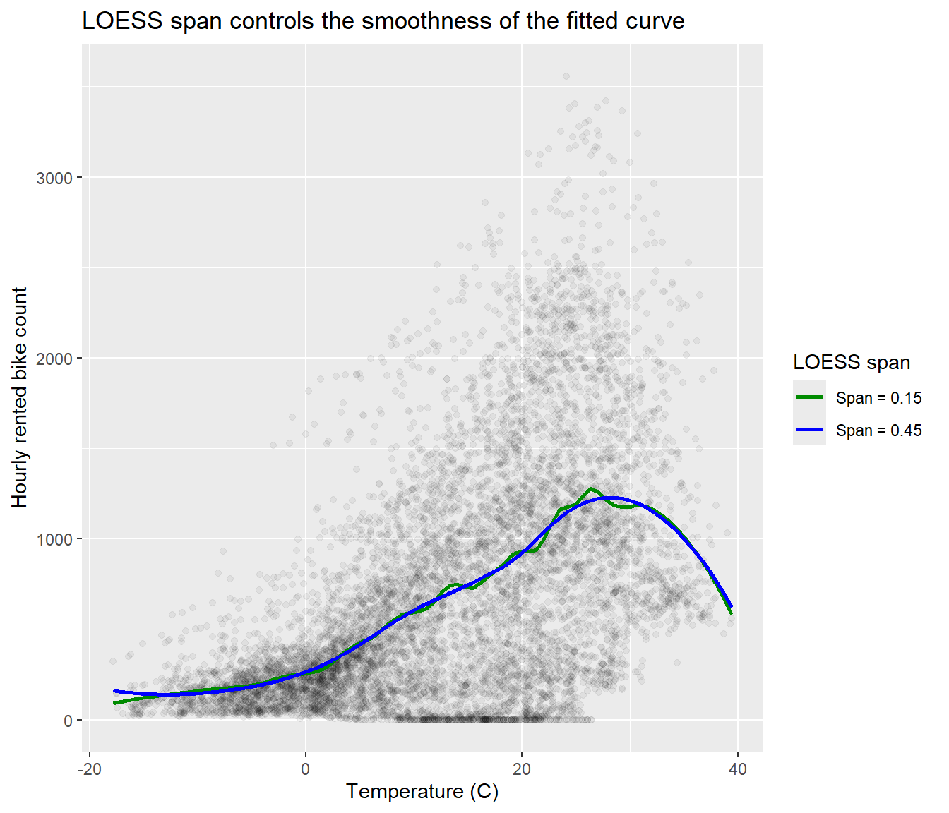
The smaller span follows local changes more closely, including random fluctuations. The larger span smooths those fluctuations but may miss a sharp change in the mean. Let’s check which features persist across both curves before choosing a regression formula.
The animation keeps the observations fixed and changes only the span. Watch what happens to the smaller local features as each fit borrows information from farther away.

31.5 From Piecewise Lines to Cubic Splines
We have already seen the basic idea behind a spline. In Lecture 18, a piecewise linear model with one knot at \(\kappa\) was
\[ f(x)=\beta_0+\beta_1x+\beta_2(x-\kappa)_+. \]
The extra term is zero before the knot and changes the slope after it. The lines join, but there can be a sharp corner at the knot.
A cubic spline uses the same piecewise idea with cubic curves. One way to write a cubic spline with knots \(\kappa_1,\ldots,\kappa_K\) is
\[ f(x)=\beta_0+\beta_1x+\beta_2x^2+\beta_3x^3 +\sum_{j=1}^{K}\gamma_j(x-\kappa_j)_+^3. \]
Each new term is zero before its knot. At the knot, \((x-\kappa)_+^3\) and its first two derivatives are all zero. The new cubic piece can therefore change the shape after the knot without introducing a jump, a corner, or an abrupt change in curvature.
So a cubic spline is simply piecewise cubic, with the pieces joined smoothly. We use the equation to understand the construction; we do not need to calculate these coefficients by hand.
31.6 Fitting a Cubic Spline in R
R’s bs() function constructs the terms needed to fit a cubic spline. Cubic is the default, so
fits a cubic spline, not a fifth-degree polynomial.
For a cubic spline fitted with the default intercept = FALSE,
\[ \text{number of internal knots} = df - 3. \]
So df = 5 gives two internal knots. Increasing the degrees of freedom keeps the pieces cubic but adds more internal knots, giving the curve more places where its curvature can adapt.
31.7 Degrees of Freedom and Flexibility
The animation holds the data and the cubic degree fixed. Only the degrees of freedom change: df = 4, 5, 8, 10. The dashed lines mark the internal knots. As df increases, the spline gains more knots and can adapt its curvature in more places.

More flexibility is not automatically better. A larger df will usually follow the observed data more closely, but it also gives the fitted mean more opportunity to follow random variation.
31.8 Cubic and Natural Cubic Splines
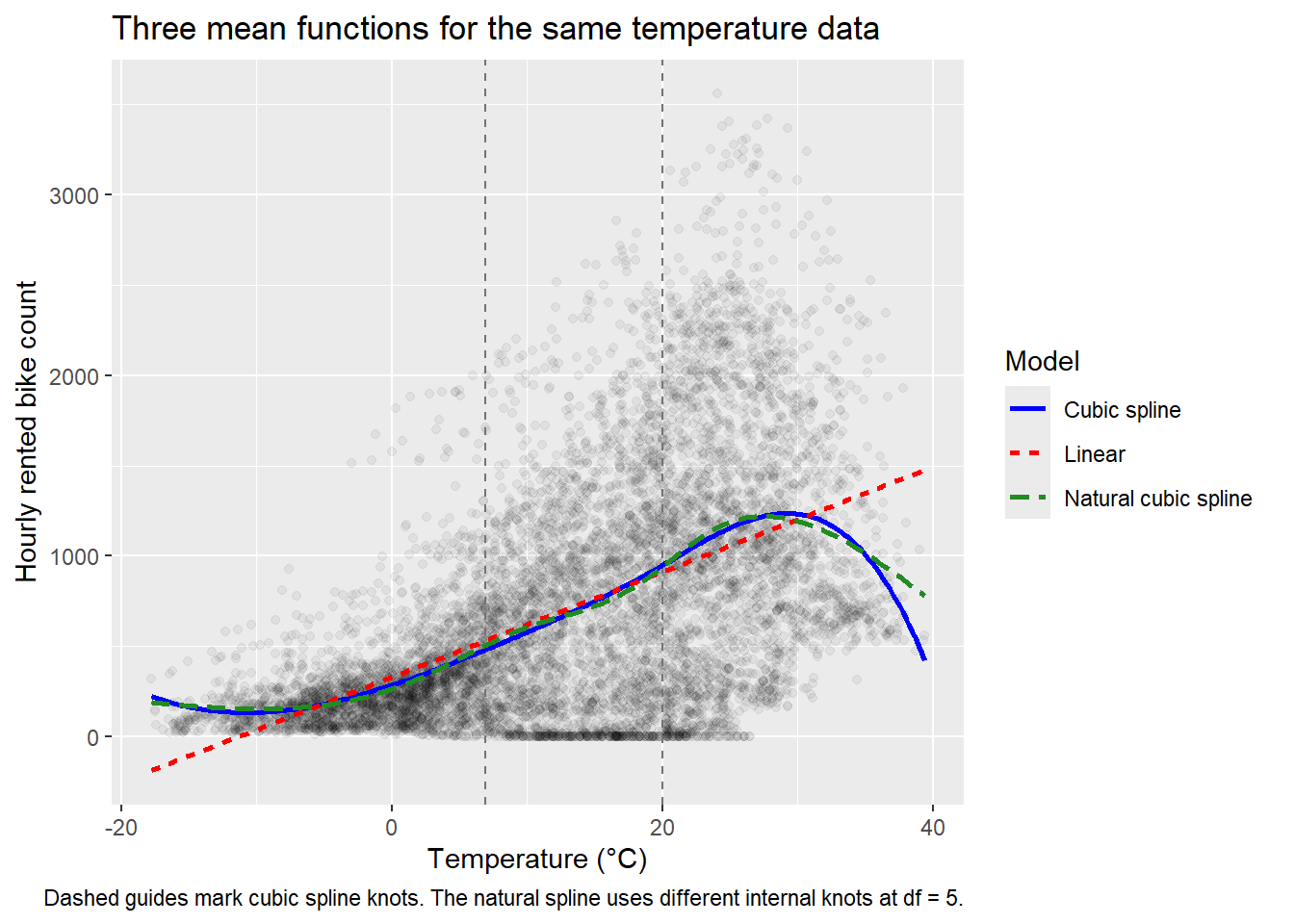
Now compare three mean functions for exactly the same temperature data: a straight line, an ordinary cubic spline, and a natural cubic spline. Both spline fits use df = 5.
lm_cubic_spline <- lm(
  rented_bike_count ~ bs(temperature, df = 5),
  data = seoul_temp
)

lm_natural_spline <- lm(
  rented_bike_count ~ ns(temperature, df = 5),
  data = seoul_temp
)
The two R functions use different constructions internally, so the same df does not imply identical internal knot locations. What matters here is the difference in the fitted curves, especially near the boundaries.
31.9 Natural Splines at the Boundaries
A cubic regression spline can keep curving beyond the temperatures we observed. A natural cubic spline is cubic through the data but is defined to have linear tails beyond its boundary knots, \(a\) and \(b\). Its curvature is zero where those tails begin:
\[ f''(a)=0 \qquad\text{and}\qquad f''(b)=0. \]
The middle of the fitted curve can still bend. The boundary rule limits what happens at the edges, where the data give us the least guidance.
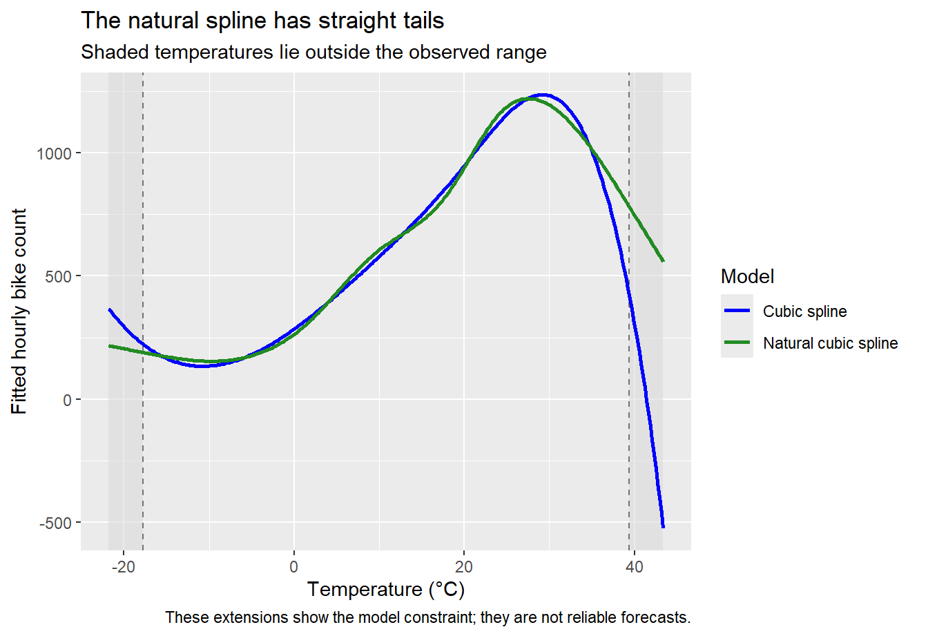
The ordinary cubic spline can continue curving; the natural cubic spline is straight beyond each boundary. Linear tails prevent one kind of unstable extension, but they do not provide information about bike demand at unobserved temperatures. A flexible curve will also tend to fit the observed data more closely, which alone does not make it the better model.
31.10 Where Does the Flexibility Come From?
| Method | Building blocks or fitting rule | Where shape can change |
|---|---|---|
| Straight line | \(1,x\) | One slope everywhere |
| Cubic polynomial | \(1,x,x^2,x^3\) | One global cubic curve |
| Piecewise linear | Line plus hinge terms | Slope changes at knots |
| Cubic spline | Smoothly joined cubic pieces | Curvature can change around knots |
| Natural cubic spline | Smoothly joined cubic pieces with linear tails | Curvature can change around knots; straight beyond boundaries |
| LOESS | Repeated distance-weighted regressions | Local neighbourhoods |
31.11 Comparing Models
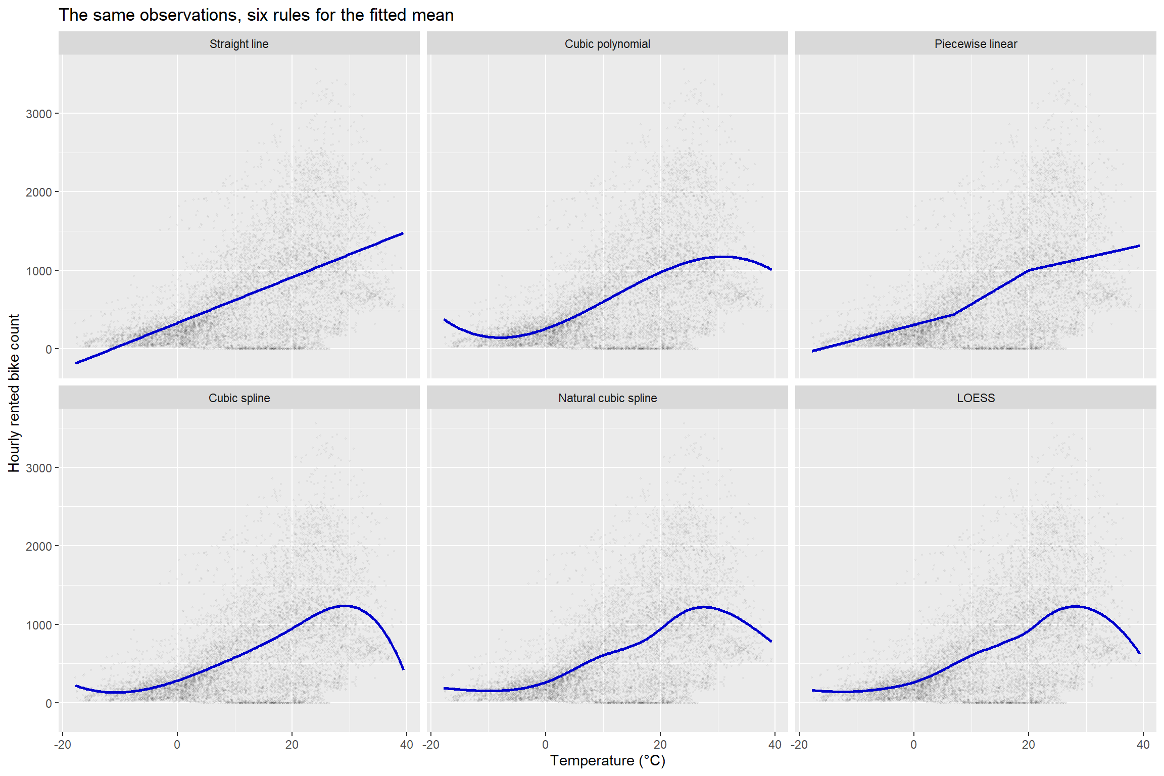
Every model below uses the same hourly Seoul observations, and every panel uses the same axes. The piecewise fit uses the same two knot locations as the df = 5 cubic spline; the LOESS fit uses span = 0.45. The polynomial is cubic, and both spline fits use df = 5.
31.12 A Second Nonlinear Signal
Temperature is not the only candidate for nonlinear modelling. Solar radiation may also have a curved relationship with demand.
seoul_hourly |>
    ggplot(aes(x = solar_radiation, y = rented_bike_count)) + geom_point(alpha = 0.05) +
    geom_smooth(method = "loess", formula = y ~ x, se = FALSE, linewidth = 1) + labs(x = "Solar radiation",
    y = "Hourly rented bike count", title = "Other weather predictors may also need flexible mean functions")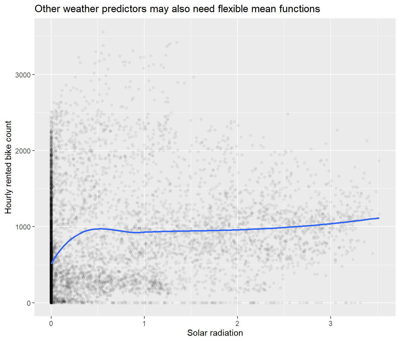
31.13 What Have We Changed? What has stayed the same?
We have changed the shape allowed for the mean response. A polynomial gives us one global curve. Piecewise regression lets the slope change at knots. Cubic splines keep the piecewise construction but join the pieces smoothly, and natural splines restrict the tails to straight lines. LOESS takes a different route: it repeatedly fits a distance-weighted local regression.
None of these choices removes the question of how much flexibility the data support. For LOESS, that choice is mainly the span. For a cubic spline, it is the number and placement of knots, which we control in R through the degrees of freedom. A close fit to these observations is not, by itself, evidence that the curve will predict new observations well.
LOESS is useful when we want to inspect the shape of a relationship without committing to one global equation. Cubic splines let us put that flexibility directly into a regression model alongside other predictors. In the next lecture, time itself enters the mean model: first through a seasonal indicator in ski sales, then through trend and seasonal terms for daily Seoul bike demand. Later we will ask whether observations close together in time can still be treated as independent.