Lecture 32 Time-Indexed Regression: Trend and Seasonality
32.1 Lectures 32/33: Time-Indexed Regression: Trend and Seasonality
The previous lectures focused on choosing predictors and flexible mean functions. We now turn to a different complication: observations collected through time.
In ordinary regression we usually write \[y_i = \beta_0 + \beta_1 x_{i1} + \cdots + \beta_p x_{ip} + \varepsilon_i,\] and assume that the errors \(\varepsilon_i\) are independent. For the moment we keep that assumption and focus on how regular time patterns can be represented in the mean of the model.
By the end of this lecture, students should be able to:
- Explain why time-indexed data often need explicit time predictors.
- Use seasonal indicators and sine/cosine pairs to represent time-of-year effects.
- Explain why fitting sine and cosine together allows an unknown phase shift.
- Use additional Fourier pairs to describe a richer seasonal shape.
- Combine trend, seasonal terms and other predictors in a regression mean model.
- Distinguish mean structure in time from residual dependence over time.
- Recognise the same modelling ideas in the ski-sales, electricity and Seoul bike examples.
32.2 Ski Sales: A First Seasonal Example
Often time series show a regular seasonal pattern. One simple way to handle this in a regression model is to create indicator variables for the most obvious seasonal effect.
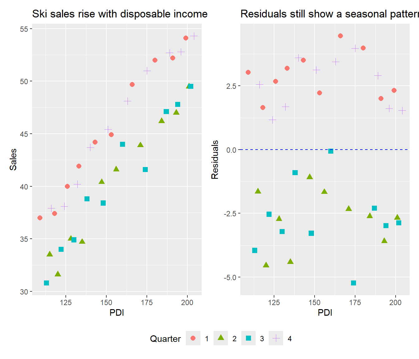
We begin with quarterly ski equipment sales and personal disposable income (PDI). Sales increase over time as income increases, but there also appears to be a seasonal pattern.
| Year | Quarter | Sales | PDI | Time |
|---|---|---|---|---|
| 1964 | 1 | 37.0 | 109 | 1964.00 |
| 1964 | 2 | 33.5 | 115 | 1964.25 |
| 1964 | 3 | 30.8 | 113 | 1964.50 |
| 1964 | 4 | 37.9 | 116 | 1964.75 |
| 1965 | 1 | 37.4 | 118 | 1965.00 |
| 1965 | 2 | 31.6 | 120 | 1965.25 |
32.3 A Winter Indicator
SkiSales <- SkiSales |>
    mutate(Winter = as.numeric(Quarter == 1 | Quarter == 4))

SkiSales_lm2 <- lm(Sales ~ PDI + Winter, data = SkiSales)
summary(SkiSales_lm2)
Call:
lm(formula = Sales ~ PDI + Winter, data = SkiSales)

Residuals:
     Min       1Q   Median       3Q      Max
-2.51118 -0.78640  0.02632  0.72842  2.67040

Coefficients:
            Estimate Std. Error t value Pr(>|t|)
(Intercept) 9.540202   0.974825   9.787 8.23e-12 ***
PDI         0.198684   0.006036  32.915  < 2e-16 ***
Winter      5.464342   0.359682  15.192  < 2e-16 ***
---
Signif. codes:  0 '***' 0.001 '**' 0.01 '*' 0.05 '.' 0.1 ' ' 1

Residual standard error: 1.137 on 37 degrees of freedom
Multiple R-squared:  0.9724,    Adjusted R-squared:  0.971
F-statistic: 652.9 on 2 and 37 DF,  p-value: < 2.2e-16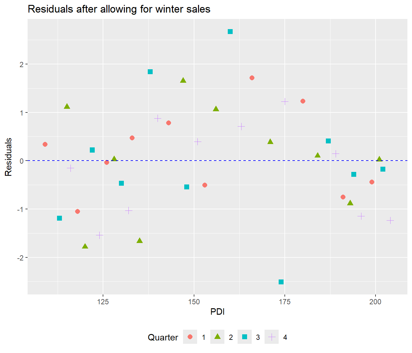
The winter indicator is strongly associated with sales, and the residuals look much less structured by quarter.
32.3.1 Is Winter Enough?
We can still ask whether there is any extra difference between the first and second half of winter, or between the two summer quarters.
SkiSales <- SkiSales |>
    mutate(Q4 = as.numeric(Quarter == 4), Q2 = as.numeric(Quarter == 2))

SkiSales_lm3 <- lm(Sales ~ PDI + Winter + Q4 + Q2, data = SkiSales)
summary(SkiSales_lm3)
Call:
lm(formula = Sales ~ PDI + Winter + Q4 + Q2, data = SkiSales)

Residuals:
     Min       1Q   Median       3Q      Max
-2.51356 -0.86028  0.03654  0.67965  2.67306

Coefficients:
             Estimate Std. Error t value Pr(>|t|)
(Intercept)  9.479913   1.037830   9.134 8.58e-11 ***
PDI          0.199044   0.006190  32.155  < 2e-16 ***
Winter       5.645220   0.520508  10.846 9.72e-13 ***
Q4          -0.353116   0.521495  -0.677    0.503
Q2           0.008279   0.519706   0.016    0.987
---
Signif. codes:  0 '***' 0.001 '**' 0.01 '*' 0.05 '.' 0.1 ' ' 1

Residual standard error: 1.162 on 35 degrees of freedom
Multiple R-squared:  0.9728,    Adjusted R-squared:  0.9697
F-statistic: 313 on 4 and 35 DF, p-value: < 2.2e-16Analysis of Variance Table
Model 1: Sales ~ PDI + Winter
Model 2: Sales ~ PDI + Winter + Q4 + Q2
Res.Df RSS Df Sum of Sq F Pr(>F)
1 37 47.864
2 35 47.245 2 0.61919 0.2294 0.7962For these data, the simple winter indicator captures the main seasonal effect well enough. This is our first example of time-indexed regression: the mean changes with both income and time-of-year.
32.4 Electricity Bills: Month Effects and Seasonal Shape
The winter indicator was enough for ski sales. With monthly observations, we can look more closely at the shape across the year. Electricity bills give us several years of data to work with.
We consider monthly electricity bills for a household from May 1994 to May 1998. During some months there were paying guests staying in part of the house, so the householder wanted to estimate the extra business-related electricity cost.
We first allow for bill length, whether the bill was estimated, guest weeks, and a time trend. Then we examine the seasonal pattern that remains.
| Bill | Days | Estimate | Guestwks | Month | Monthlab | Time | Year |
|---|---|---|---|---|---|---|---|
| 70.18 | 29 | 0 | 0 | 5 | M | 5 | 94 |
| 79.05 | 30 | 1 | 0 | 6 | J | 6 | 94 |
| 78.60 | 27 | 0 | 0 | 7 | J | 7 | 94 |
| 81.45 | 29 | 1 | 0 | 8 | A | 8 | 94 |
| 174.25 | 28 | 0 | 4 | 9 | S | 9 | 94 |
| 115.20 | 28 | 1 | 0 | 10 | O | 10 | 94 |
32.5 Electricity: Residual Seasonality After Basic Adjustment
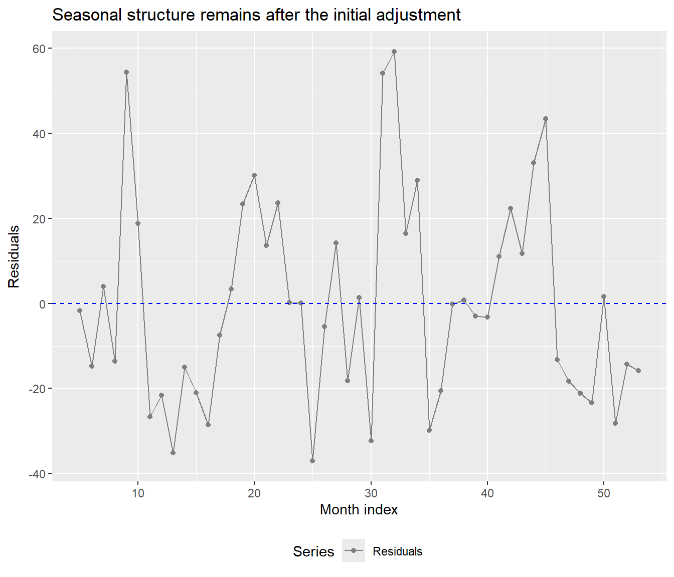
After this adjustment, residuals tend to be positive in some months and negative in others. That suggests a seasonal pattern remains.
We use the residual plot to choose seasonal terms for the mean model. To test their contribution, we add them to the original Bill regression while keeping Days, Estimate, Guestwks and Time in the model.
32.5.1 Sinusoidal Terms
A sine curve on its own fixes where the peak falls. By fitting sine and cosine together, we let the data determine that position. We use a period of 12 months here, so the seasonal component repeats each year.
32.5.2 Electricity: Moving the Sine and Cosine Curves
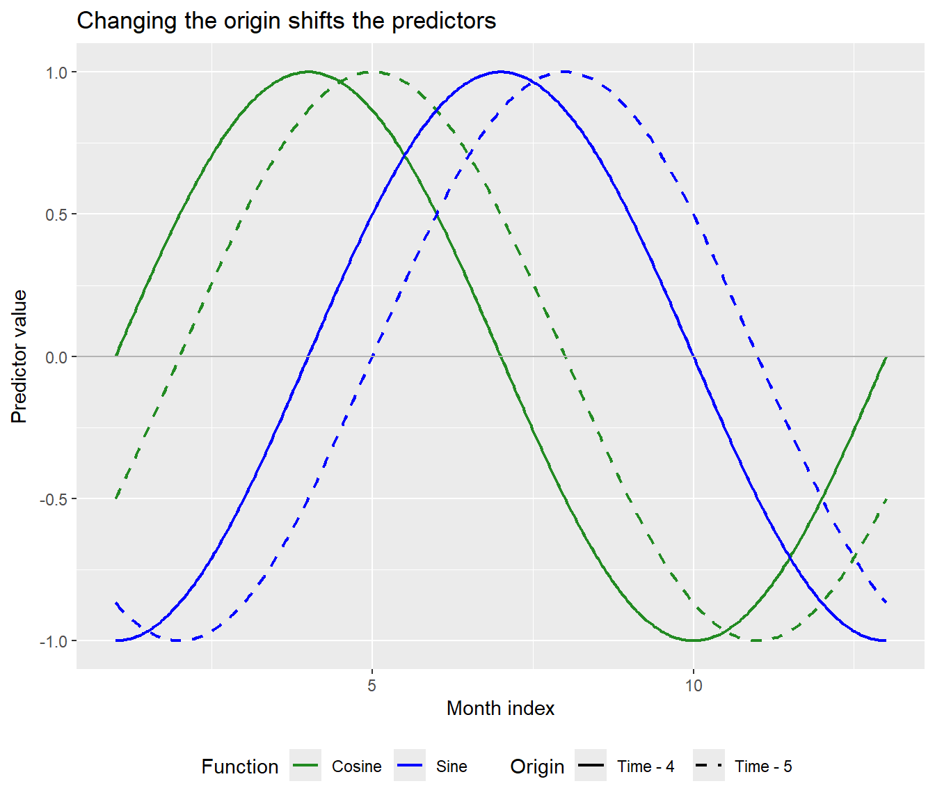
Subtracting 4 or 5 shifts the curves along the time axis. Both pairs still repeat every 12 months. At the chosen origin, sine is zero and cosine is one; moving that origin moves their zero crossings and peaks.
32.5.3 What Does Sine Plus Cosine Do?
Let’s start by giving sine and cosine a coefficient of 1 each. The red curve is their sum at each month.
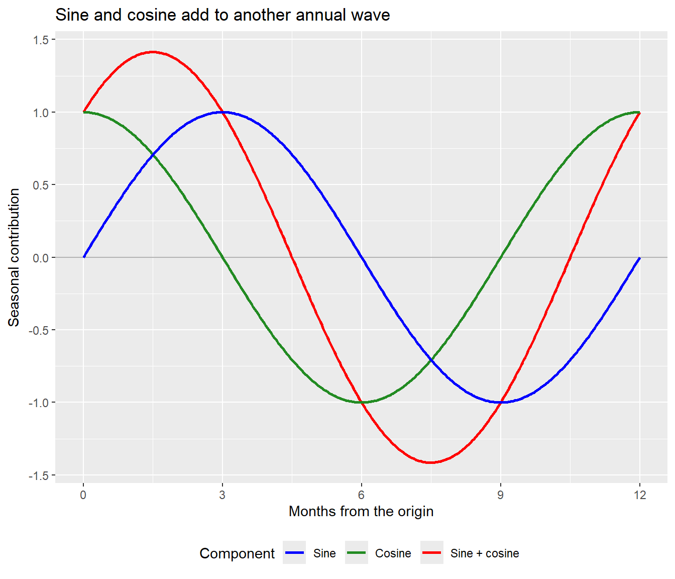
The sum still takes 12 months to repeat. Its peak lies between the two component peaks, and its amplitude is \(\sqrt{2}\) rather than 1. In a regression, we estimate the two coefficients instead of fixing them at 1. That lets the height and position of the seasonal peak change.
32.6 The Combined Wave: Amplitude and Peak Position
More generally, any weighted sum of this sine and cosine pair is another wave with the same period:
\[ b_s\sin\{\omega(t-c)\}+b_c\cos\{\omega(t-c)\} =A\sin\{\omega(t-c)+\phi\}. \]
Its amplitude is
\[ A=\sqrt{b_s^2+b_c^2}. \]
Here \(\omega=2\pi/12\) and \(c\) is the origin. The amplitude \(A\) tells us how far the seasonal component rises above and falls below zero. The phase \(\phi\) determines where its peak falls relative to that origin.
We fit \(b_s\) and \(b_c\) by ordinary linear regression. Together they let the data determine the amplitude and peak position; we do not need to fit \(A\) and \(\phi\) directly.
32.7 Electricity: Does the Starting Month Matter?
We have defined two pairs, one using Time - 4 and the other using Time - 5. Let’s fit both and see what changes.
Electricity_first4 <- lm(Bill ~ Days + Estimate + Guestwks + Time + SinTime4 + CosTime4,
    data = Electricity)
Electricity_first5 <- lm(Bill ~ Days + Estimate + Guestwks + Time + SinTime5 + CosTime5,
    data = Electricity)

Electricity <- Electricity |>
    mutate(SinTime = SinTime5, CosTime = CosTime5)
32.7.1 Same Curve, Different Coefficients
| Origin | Sine estimate | Sine P | Cosine estimate | Cosine P |
|---|---|---|---|---|
| Time - 4 | 23.477 | <0.001 | -16.276 | <0.001 |
| Time - 5 | 28.469 | <0.001 | -2.357 | 0.541 |
[1] 5.684342e-14The table shows coefficient estimates. The calculation above compares the predicted bills, using all the model terms, and shows that they agree to numerical precision. The cosine coefficient and its P-value change when we move the origin, but so do the sine coefficient and the curves they multiply.
32.8 Electricity: Same Prediction, Different Coefficients
Let’s check the seasonal contribution at Time = 5 using the coefficients in the table.
With origin 4, Time - 4 = 1, so sine is \(\sin(2\pi/12)=0.5\) and cosine is \(\cos(2\pi/12)\approx0.8660\). Their weighted sum is
\[ 23.477(0.5) -16.276(0.8660) \approx -2.357. \]
With origin 5, Time - 5 = 0, so sine is zero and cosine is one:
\[ 28.469(0) -2.357(1) = -2.357. \]
The cosine coefficients differ, but the two weighted sums agree. Both reduce the predicted bill by about 2.36 dollars through the seasonal terms. That is the seasonal contribution, not the whole predicted bill. The other model terms are unchanged too, so both models predict the same bill.
We will use origin 5 from here on. That is a convenient choice, not a better fit: retaining both terms lets either origin describe the same seasonal curve.
32.9 Electricity: Adding the Weighted Curves
Here we repeat the previous calculation across a whole year. Blue is the fitted sine contribution, green is the fitted cosine contribution, and red is their sum. Each component is its predictor curve multiplied by its estimated coefficient.
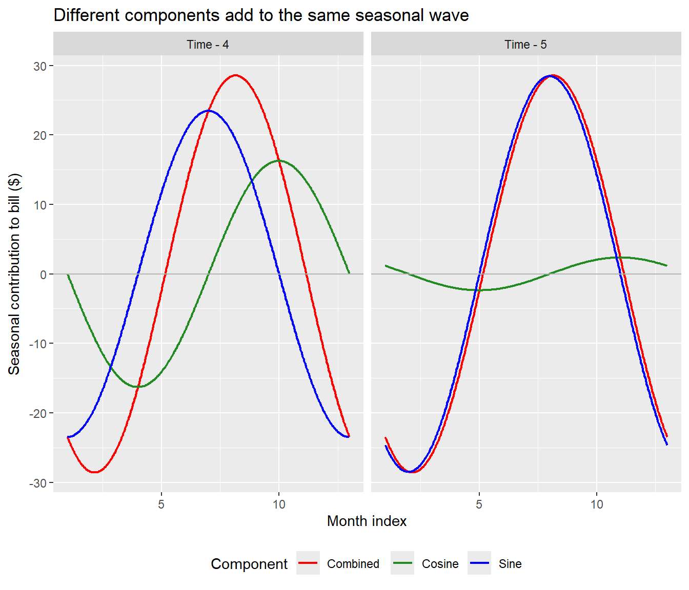
Look at the green curve on the right: it is almost flat. With origin 5, sine does most of the work. With origin 4, the seasonal adjustment is spread more across the two components.
We moved the starting point of both predictors, so the regression used different coefficients to build the same annual wave. With both terms available, either origin can describe that wave, so the best fitted sum stays the same. Compare red at any month: it agrees in both panels, even though blue and green have changed.
Red is the seasonal adjustment. We add it to the intercept and the other model terms to get the fitted bill.
32.10 Should We Keep Both Terms?
When the seasonal peak is unknown, we keep sine and cosine together and assess the pair jointly. An individual P-value asks whether one component is needed given the other, using the origin we happened to choose. It does not test whether the seasonal wave as a whole is needed.
We compare the original adjustment model with the model containing the pair: \[H_0:b_s=b_c=0.\]
Analysis of Variance Table

Model 1: Bill ~ Days + Estimate + Guestwks + Time
Model 2: Bill ~ Days + Estimate + Guestwks + Time + SinTime5 + CosTime5
  Res.Df   RSS Df Sum of Sq      F    Pr(>F)
1     44 28202
2     42 13524  2     14678 22.793 1.982e-07 ***
---
Signif. codes:  0 '***' 0.001 '**' 0.01 '*' 0.05 '.' 0.1 ' ' 1
Under the usual OLS error assumptions, this gives \(F(2,42)=22.79\), with \(p<0.001\). There is evidence for the pair even though the cosine P-value is large at the origin 5. We do not drop cosine on that basis. Using just one component restricts where the peak can fall, so that restriction needs a separate justification before looking at these P-values. If the pair is not needed, we can consider removing it together.
32.11 Electricity: What Remains After One Pair?
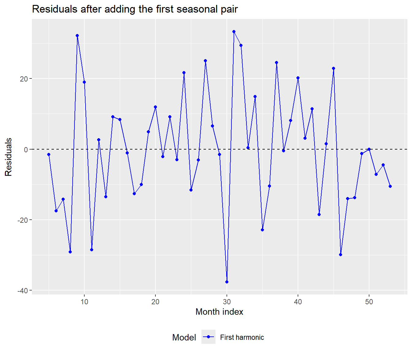
The first pair accounts for much of the recurring rise and fall. We can still see departures from that smooth wave. Let’s ask whether a second pair helps describe them.
32.12 Electricity: A Sharper Seasonal Shape
One sine/cosine pair produces a smooth cycle with one peak and one trough per year. The residual pattern suggests a sharper rise or fall than this pair can produce. Adding a second pair, at twice the frequency, allows that shape to change while keeping the original adjustment variables in the model. Compare the model with the first pair against the model with both pairs. The partial F test asks whether those two additional coefficients improve the fit after the other terms have already been included.
Electricity <- Electricity |>
    mutate(Sin2Time = sin((Time - 5) * 4 * pi/12), Cos2Time = cos((Time - 5) * 4 *
        pi/12))

Electricity_full1 <- lm(Bill ~ Days + Estimate + Guestwks + Time + SinTime + CosTime,
    data = Electricity)
Electricity_full2 <- lm(Bill ~ Days + Estimate + Guestwks + Time + SinTime + CosTime +
    Sin2Time + Cos2Time, data = Electricity)

anova(Electricity_full1, Electricity_full2)
Analysis of Variance Table
Model 1: Bill ~ Days + Estimate + Guestwks + Time + SinTime + CosTime
Model 2: Bill ~ Days + Estimate + Guestwks + Time + SinTime + CosTime +
Sin2Time + Cos2Time
Res.Df RSS Df Sum of Sq F Pr(>F)
1 42 13524
2 40 11350 2 2173.9 3.8307 0.03005 *
---
Signif. codes: 0 '***' 0.001 '**' 0.01 '*' 0.05 '.' 0.1 ' ' 1Under the usual OLS error assumptions, the second harmonic provides evidence of additional seasonal shape in these data: \(F(2, 40) = 3.83\), \(p = 0.0301\). This two-degree-of-freedom test compares models with the same original adjustment variables. In Lecture 34 we check whether residual errors are dependent, which matters for that P-value.
32.13 Electricity: Comparing the Seasonal Fits
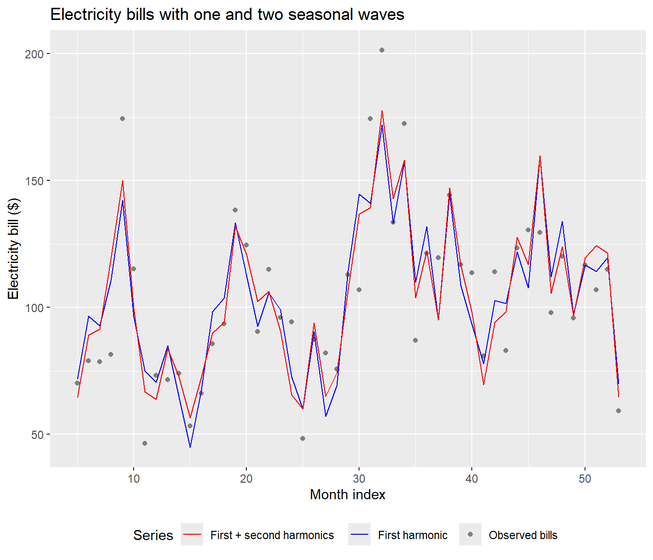
These fitted curves include the bill-length, estimated-bill, guest-week and trend adjustments as well as the seasonal terms. They describe this household after adjustment for the recorded covariates; they do not establish that the same pattern applies elsewhere.
32.14 Electricity: Comparing the Residuals
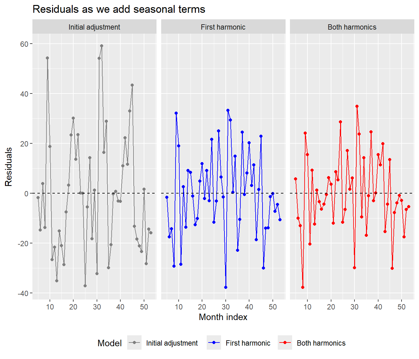
The panels use the same observations and vertical scale. They show what each step leaves behind. Smaller residuals do not establish independence, so we still need to examine how nearby deviations are related.
32.15 Electricity: Putting the Model Together
Call:
lm(formula = Bill ~ Days + Estimate + Guestwks + Time + SinTime +
    CosTime + Sin2Time + Cos2Time, data = Electricity)

Residuals:
    Min      1Q  Median      3Q     Max
-37.718  -9.495  -0.918   9.350  34.942

Coefficients:
            Estimate Std. Error t value Pr(>|t|)
(Intercept)  24.2994    35.3845   0.687   0.4962
Days          1.6721     1.2801   1.306   0.1989
Estimate     10.6697     7.0672   1.510   0.1390
Guestwks     11.0988     1.5241   7.282 7.62e-09 ***
Time          0.1432     0.1984   0.722   0.4745
SinTime      27.0035     4.0213   6.715 4.68e-08 ***
CosTime      -1.5594     3.6114  -0.432   0.6682
Sin2Time     -6.1630     3.4560  -1.783   0.0821 .
Cos2Time     -7.5589     3.6172  -2.090   0.0430 *
---
Signif. codes:  0 '***' 0.001 '**' 0.01 '*' 0.05 '.' 0.1 ' ' 1

Residual standard error: 16.84 on 40 degrees of freedom
Multiple R-squared:  0.7882,    Adjusted R-squared:  0.7458
F-statistic:  18.6 on 8 and 40 DF,  p-value: 2.985e-11
The final model is still a regression model. It adjusts for the bill length, estimated status, guest weeks and time trend, then adds smooth seasonal waves rather than a separate effect for each month.
32.16 A Modern Comparison: Daily Seoul Bike Demand
We now bring these ideas together with the daily Seoul bike data. We will first check what the observations measure, then compare a trend, a natural spline and a Fourier seasonal wave before adding weather predictors.
seoul_daily <- read_csv("../data/seoul_bike_daily.csv", show_col_types = FALSE) |>
    mutate(date = as.Date(date)) |>
    arrange(date)

seoul_daily |>
    head() |>
kable()| date | day_index | rented_bike_count | mean_temperature | mean_humidity | mean_wind_speed | mean_visibility | mean_dew_point_temperature | total_solar_radiation | total_rainfall | total_snowfall | season | holiday_any | functioning_day_all |
|---|---|---|---|---|---|---|---|---|---|---|---|---|---|
| 2017-12-01 | 1 | 9539 | -2.4541667 | 45.87500 | 1.5375000 | 1870.750 | -13.545833 | 5.97 | 0.0 | 0.0 | Winter | no | yes |
| 2017-12-02 | 2 | 8523 | 1.3250000 | 61.95833 | 1.7125000 | 1471.083 | -5.716667 | 6.33 | 0.0 | 0.0 | Winter | no | yes |
| 2017-12-03 | 3 | 7222 | 4.8750000 | 81.54167 | 1.6125000 | 455.750 | 1.883333 | 3.01 | 4.0 | 0.0 | Winter | no | yes |
| 2017-12-04 | 4 | 8729 | -0.3041667 | 52.50000 | 3.4500000 | 1362.833 | -9.925000 | 6.79 | 0.1 | 0.0 | Winter | no | yes |
| 2017-12-05 | 5 | 8307 | -4.4583333 | 36.41667 | 1.1083333 | 1959.458 | -17.425000 | 0.86 | 0.0 | 0.0 | Winter | no | yes |
| 2017-12-06 | 6 | 6669 | 0.0458333 | 70.79167 | 0.6958333 | 1186.875 | -5.187500 | 6.14 | 1.3 | 8.6 | Winter | no | yes |
32.17 Bikes: Daily Demand Before Filtering
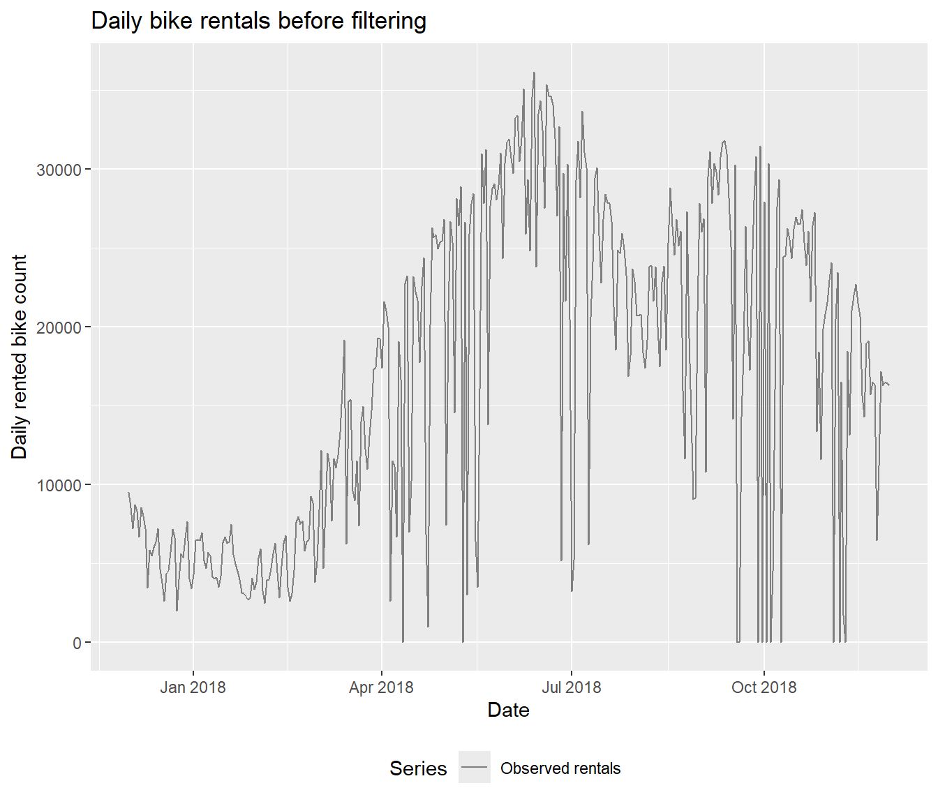
Several days drop right down to zero. Before fitting a model, let’s go back to the data and check what happened on those days.
32.18 Bikes: Checking the Non-Functioning Days
The functioning_day_all variable records whether the bike system was functioning throughout the day. Let’s count the days that are not marked "yes".
[1] 13There are 12 days with zero rentals, but 13 days marked as not functioning all day. One of those days still recorded some rentals. We use the functioning-day flag to identify the days to exclude.
32.19 Bikes: Demand on Functioning Days
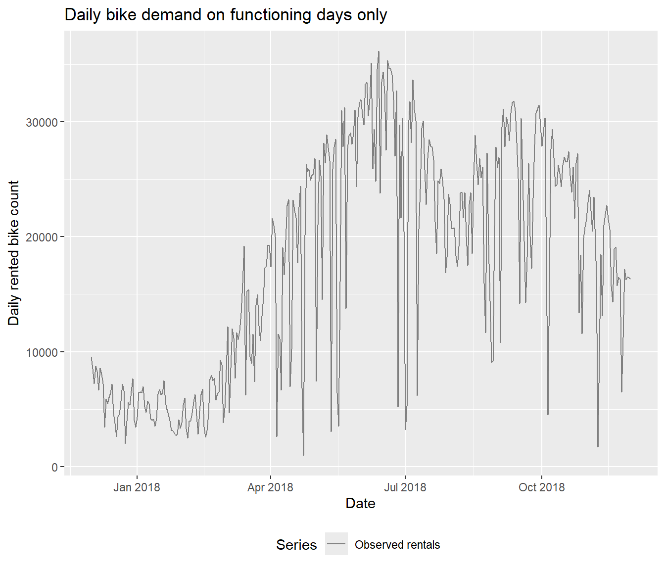
On the excluded days, the rental count also reflects restricted access to bikes, so those days do not measure ordinary demand.
We removed 13 outage days. The remaining rows retain their original dates and day_index values, so consecutive rows are not always consecutive days. Keep that distinction in mind when we examine residual dependence.
This dataset covers one year. Its rise and fall within that year are visible, but one year cannot establish that the same annual cycle will recur or that a fitted linear trend persists over several years.
32.20 Bikes: Trend-Only Model
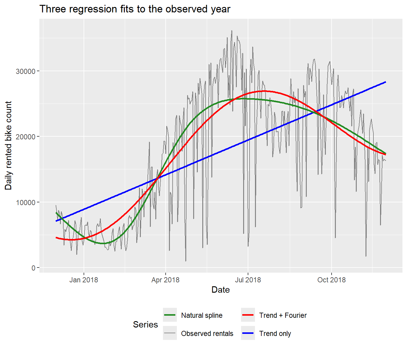
A linear trend captures the broad direction but ignores the seasonal pattern entirely.
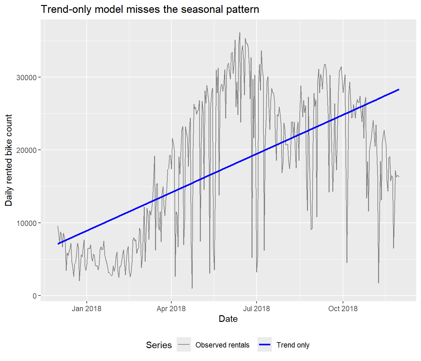
The fitted line describes a broad change across the observed year, but it misses the rise and fall within that year. It underpredicts in some parts of the year and overpredicts in others, as we also saw in the ski sales residuals.
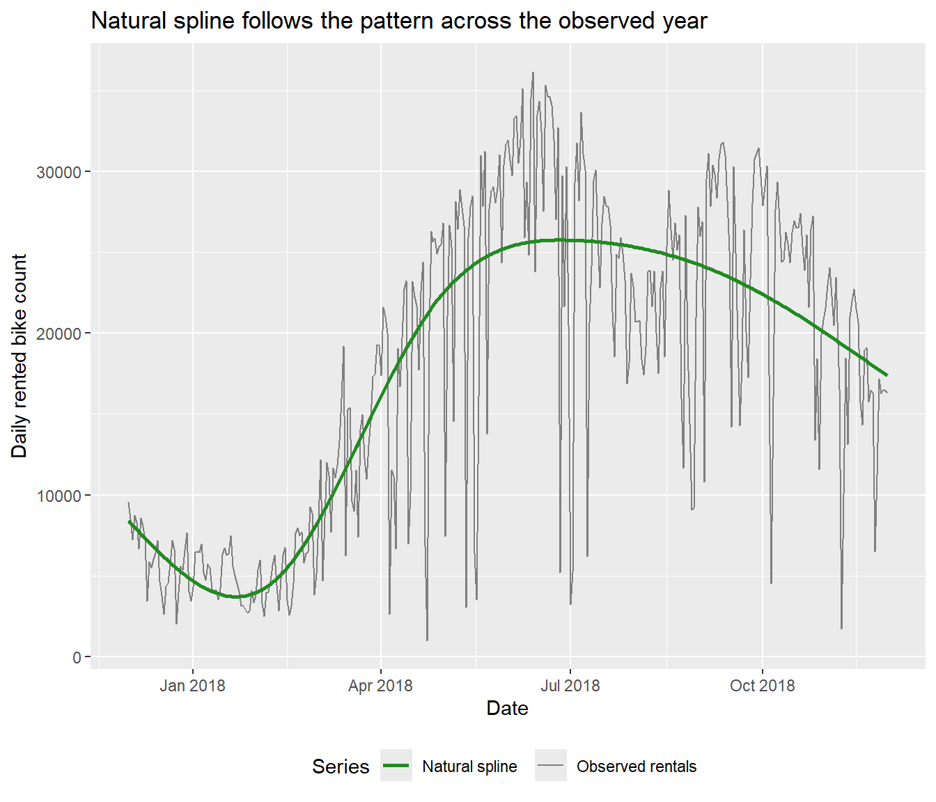
32.21 Bikes: Fitting a Natural Spline Through Time
Last lecture we used natural splines to fit a curved relationship with temperature. We can do the same thing with time. We keep df = 5 here and let the fitted mean bend across the year.
32.22 Bikes: Adding a Fourier Seasonal Term
A sine and cosine pair with a one-year period describes a smooth within-year pattern without needing a separate indicator for each date.
We use the same sine and cosine pair as in the electricity example, now with a period of 365 days. Fitting the pair together lets the data determine where the seasonal peak falls. These predictors are called Fourier terms, and they add two coefficients to the trend-only model.
The spline lets the mean bend across the dates we observed, but it does not require that shape to repeat. A sine and cosine pair defines a wave that repeats every 365 days, so it is a natural choice when we expect a seasonal pattern to recur. The linear trend can still move the overall level up or down from year to year; it is the seasonal component that repeats.
seoul_daily_clean <- seoul_daily_clean |>
    mutate(S1 = sin(2 * pi * day_index/365), C1 = cos(2 * pi * day_index/365))

seoul_fourier <- lm(rented_bike_count ~ day_index + S1 + C1, data = seoul_daily_clean)
summary(seoul_fourier)
Call:
lm(formula = rented_bike_count ~ day_index + S1 + C1, data = seoul_daily_clean)

Residuals:
     Min       1Q   Median       3Q      Max
-23326.8  -2884.9    664.6   4330.8  10705.3

Coefficients:
            Estimate Std. Error t value Pr(>|t|)
(Intercept) 11292.21     930.79  12.132  < 2e-16 ***
day_index      34.54       4.82   7.166 4.64e-12 ***
S1          -4292.64     714.83  -6.005 4.81e-09 ***
C1          -6652.94     450.80 -14.758  < 2e-16 ***
---
Signif. codes:  0 '***' 0.001 '**' 0.01 '*' 0.05 '.' 0.1 ' ' 1

Residual standard error: 5988 on 348 degrees of freedom
Multiple R-squared:  0.641, Adjusted R-squared:  0.6379
F-statistic: 207.1 on 3 and 348 DF,  p-value: < 2.2e-16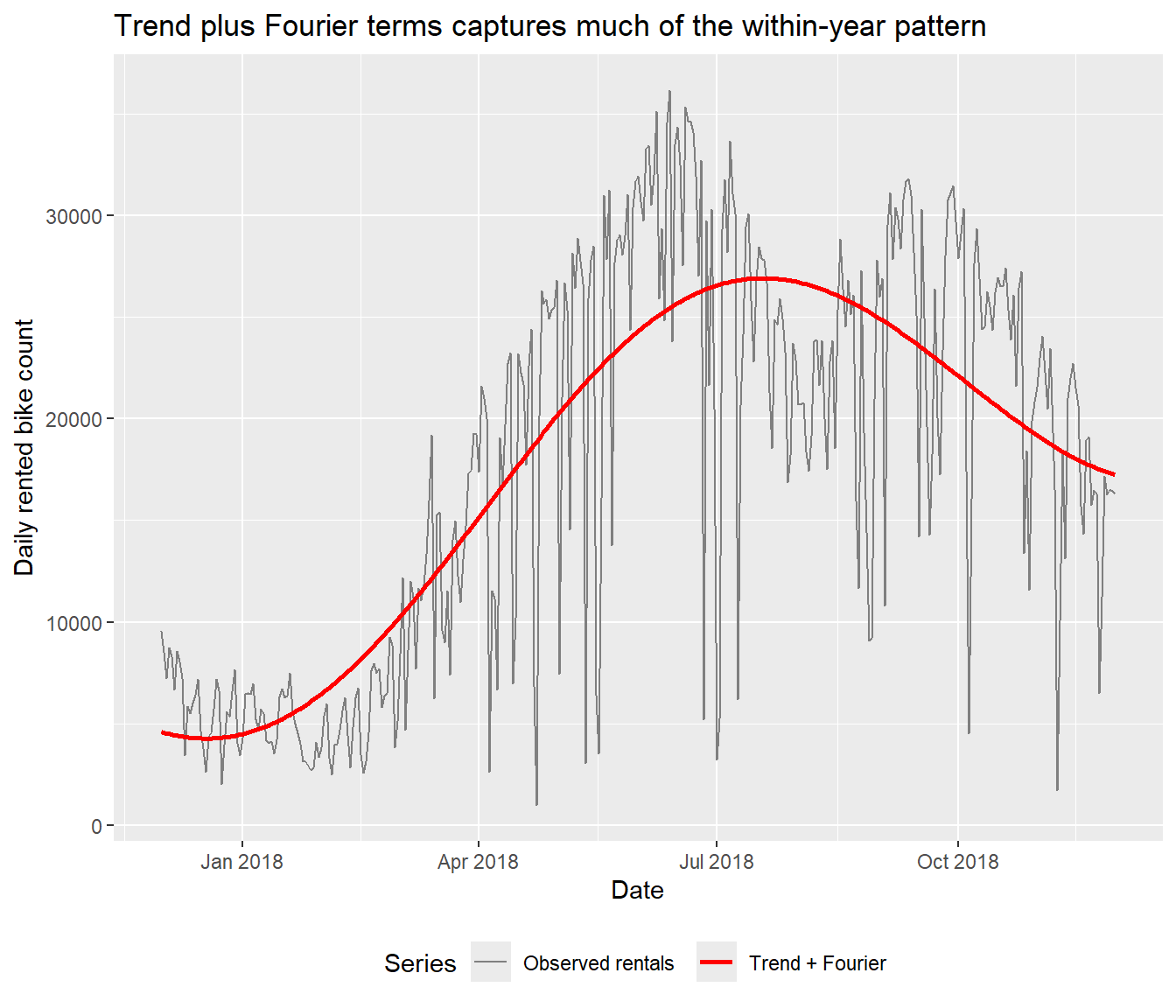
The Fourier pair adds only two parameters and captures much of the observed rise and fall. We have a one-year record, so this fitted cycle describes the pattern within these data; it does not establish that the same pattern will recur in later years.
32.23 Bikes: Comparing Trend, Natural Spline and Fourier Fits
We can now compare three ways of describing the mean through time: a straight line, a natural spline, and a trend with an annual sine and cosine pair.
| Model | \(R^2\) |
|---|---|
| Trend only | 0.377 |
| Natural spline | 0.668 |
| Trend + Fourier | 0.641 |
All three fits use ordinary regression on the same functioning days. The straight line gives a constant rate of change, the natural spline lets the mean bend through time, and the Fourier pair adds an annual wave to the trend. A closer fit to these observations alone does not tell us which model will predict future demand best.
32.24 Bikes: Adding Weather and a Second Fourier Pair
The three fits above describe how demand changes through time. We also recorded temperature, rainfall and solar radiation, so we can include those predictors alongside the seasonal terms. We add a second Fourier pair, just as we did for electricity, to allow a richer within-year shape.
seoul_daily_clean <- seoul_daily_clean |>
    mutate(S2 = sin(4 * pi * day_index/365), C2 = cos(4 * pi * day_index/365))

seoul_full <- lm(rented_bike_count ~ day_index + S1 + C1 + S2 + C2 + mean_temperature +
    total_rainfall + total_solar_radiation, data = seoul_daily_clean)
summary(seoul_full)
Call:
lm(formula = rented_bike_count ~ day_index + S1 + C1 + S2 + C2 +
    mean_temperature + total_rainfall + total_solar_radiation,
    data = seoul_daily_clean)

Residuals:
     Min       1Q   Median       3Q      Max
-12080.9  -1929.8    283.4   2181.2  10819.9

Coefficients:
                       Estimate Std. Error t value Pr(>|t|)
(Intercept)            8909.822   1125.618   7.915 3.44e-14 ***
day_index                12.678      3.798   3.338 0.000938 ***
S1                    -4481.066    801.992  -5.587 4.70e-08 ***
C1                    -3293.777    733.285  -4.492 9.66e-06 ***
S2                    -2279.788    356.157  -6.401 5.07e-10 ***
C2                     2620.035    288.115   9.094  < 2e-16 ***
mean_temperature        147.934     57.435   2.576 0.010422 *
total_rainfall         -221.150     20.975 -10.543  < 2e-16 ***
total_solar_radiation   387.995     41.268   9.402  < 2e-16 ***
---
Signif. codes:  0 '***' 0.001 '**' 0.01 '*' 0.05 '.' 0.1 ' ' 1

Residual standard error: 3643 on 343 degrees of freedom
Multiple R-squared:  0.869, Adjusted R-squared:  0.8659
F-statistic: 284.4 on 8 and 343 DF,  p-value: < 2.2e-16
32.25 Bikes: The Combined Fit
The full model has \(R^2 = 0.869\) on these 352 functioning days.
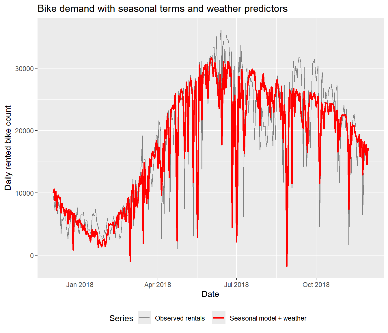
This model includes both a more flexible seasonal shape and the recorded weather predictors. Its difference from the earlier Fourier fit reflects all those additions together. We still have only one year of observations, so the seasonal terms describe the observed pattern without establishing that it will recur.
32.26 Bikes: What Remains After the Combined Fit?
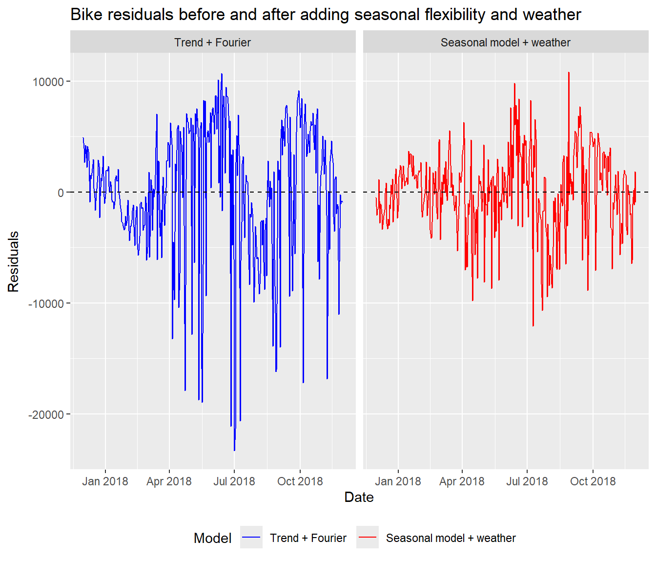
We have added both a second seasonal pair and weather predictors, so the change reflects all those additions. The residuals are smaller, but nearby days can still show similar departures from the fitted mean. Lecture 34 looks more closely at that dependence. The dates still contain gaps where outage days were excluded; neighbouring rows are not always neighbouring days.
32.27 Lecture Summary
We are still using ordinary regression. We have added predictors that describe when an observation was collected, alongside the other variables that help explain the response.
For ski sales, income got us part of the way, but a winter indicator was needed to account for the differences between quarters. With electricity bills, we used sine and cosine together to let the seasonal peak fall anywhere in the year. Changing the origin changed their coefficients and individual P-values without changing the fitted curve, so we assessed sine and cosine together. A second pair gave us more flexibility in the seasonal shape.
The bike data brought those ideas together. We checked the outage days, compared a straight-line trend, a natural spline and a Fourier wave, then fitted a richer model with a second pair and weather predictors. The spline lets the mean bend through the observed year; the Fourier terms define seasonal waves that repeat. One year of bike data cannot establish that those waves will recur or that the trend will continue.
32.27.1 Mean Structure First, Error Dependence Later
Across these examples we used time predictors to describe the mean response: \[E(Y_t) = \beta_0 + \beta_1 t + \beta_2 z_t + \cdots.\]
That is different from saying the errors are autocorrelated. A model can capture clear time structure in the mean and still leave dependent residuals behind. Lecture 34 takes the richer bike model forward and asks whether the residuals behave independently.