Lecture 27 Automatic Model Selection
27.1 Model Selection using AIC
An alternative approach to selecting a good model is to define a measure of the quality of a model, then choose the model with the highest quality.
A common measure of quality is the Akaike Information Criterion (AIC).
27.2 Information Criteria
A good regression model (i.e. with a good choice of predictors) will:
- fit the data well;
- be simple (have as few predictors as possible).
Hence quality of a model can be measured by a quantity of the form \[\mbox{Measure of badness of fit} + k \times \mbox{Number of predictors} + \mbox{constant}\]
where k can be adjusted to control the relative importance of the two aspects of a model’s quality just given.
Note that any additive constant is of no real importance, since in comparing the quality of different models (our real aim) the constant term cancels out.
27.3 Akaike Information Criterion
Several information criteria in statistics are in the form given above for a “measure of badness of fit”.
The most popular probably the Akaike Information Criterion (AIC). For a linear model with unknown error variance this is defined by \[AIC = n \log (RSS/n) + 2p + \mbox{constant}.\]
As it is a measure of badness of fit we choose the model with smallest AIC.
N.B. This is not the only criterion in common use, but is perhaps the most common. Different software present different criteria.
27.4 Back to the Climate data
In the previous topic we found two different models, climate.lm6 and climate.s2. These not only have different numbers of variables, but are not even nested! However we can compare them using the adjusted R-square, or the function AIC(). Both criteria suggest that the model lm6 is to be preferred.
climate = read.csv("../../data/Climate.csv", header = TRUE, row.names = 1)
climate.lm6 = lm(Sun ~ Long + MnJanTemp + NorthIsland, data = climate)
climate.s2 = lm(Sun ~ MnJanTemp + Rain, data = climate)
summary(climate.lm6)$adj.r.square
[1] 0.4023174summary(climate.s2)$adj.r.square[1] 0.3530486AIC(climate.lm6)[1] 476.4903AIC(climate.s2)[1] 478.4497An alternative to AIC() is the extractAIC() command. The output from extractAIC() command is number of regression
parameters (p+1) and the model’s AIC.
extractAIC(climate.lm6)[1] 4.0000 372.3268extractAIC(climate.s2)[1] 3.0000 374.286127.5 AIC in Stepwise Variable Selection
We have seen that sequential variable selection can be conducted using a sequence of F tests.
An alternative is to compare models using AIC.
Specifically, at each step of the algorithm we change to the model with smallest AIC (from adding or dropping a single variable), and stop only when we cannot reduce AIC by single term additions or deletions.
This procedure is implemented using the step() command in R. The following performs stepwise selection starting with the null model. Note the scope option gives the maximum possible model.
climate.null = lm(Sun ~ 1, data = climate)
climate.step <- step(climate.null, scope = ~Lat + Long + MnJanTemp + MnJlyTemp +
    Height + Rain + Sea + NorthIsland, data = climate, direction = "both")
Start: AIC=388.08
Sun ~ 1
Df Sum of Sq RSS AIC
+ MnJanTemp 1 506057 1130350 376.76
+ Long 1 344588 1291820 381.57
+ Rain 1 316258 1320150 382.35
+ Lat 1 220053 1416355 384.88
+ MnJlyTemp 1 182734 1453674 385.82
+ Sea 1 148252 1488156 386.66
+ NorthIsland 1 95788 1540620 387.91
+ Height 1 90941 1545467 388.02
<none> 1636408 388.08
Step: AIC=376.76
Sun ~ MnJanTemp
Df Sum of Sq RSS AIC
+ Rain 1 132170 998181 374.29
+ NorthIsland 1 76944 1053407 376.22
<none> 1130350 376.76
+ Sea 1 50284 1080066 377.12
+ Lat 1 43712 1086639 377.34
+ MnJlyTemp 1 22898 1107452 378.03
+ Long 1 14102 1116248 378.31
+ Height 1 40 1130310 378.76
- MnJanTemp 1 506057 1636408 388.08
Step: AIC=374.29
Sun ~ MnJanTemp + Rain
Df Sum of Sq RSS AIC
+ Sea 1 87195 910985 373.00
<none> 998181 374.29
+ NorthIsland 1 53140 945040 374.32
+ Long 1 12081 986099 375.85
+ Height 1 1193 996988 376.24
+ Lat 1 330 997850 376.27
+ MnJlyTemp 1 16 998165 376.29
- Rain 1 132170 1130350 376.76
- MnJanTemp 1 321969 1320150 382.35
Step: AIC=373
Sun ~ MnJanTemp + Rain + Sea
Df Sum of Sq RSS AIC
+ Height 1 94788 816197 371.04
+ MnJlyTemp 1 52902 858083 372.84
<none> 910985 373.00
+ Long 1 38986 871999 373.42
- Sea 1 87195 998181 374.29
+ NorthIsland 1 16393 894592 374.34
+ Lat 1 1945 909040 374.92
- Rain 1 169081 1080066 377.12
- MnJanTemp 1 214016 1125001 378.59
Step: AIC=371.04
Sun ~ MnJanTemp + Rain + Sea + Height
Df Sum of Sq RSS AIC
<none> 816197 371.04
+ NorthIsland 1 28556 787641 371.76
+ MnJlyTemp 1 22773 793424 372.02
+ Long 1 19420 796777 372.17
+ Lat 1 10788 805409 372.56
- Height 1 94788 910985 373.00
- Sea 1 180791 996988 376.24
- Rain 1 226572 1042769 377.86
- MnJanTemp 1 284136 1100333 379.79summary(climate.step)
Call:
lm(formula = Sun ~ MnJanTemp + Rain + Sea + Height, data = climate)

Residuals:
    Min      1Q  Median      3Q     Max
-268.06 -104.31    1.62   90.67  344.42

Coefficients:
            Estimate Std. Error t value Pr(>|t|)
(Intercept) 872.1199   356.7010   2.445  0.02037 *
MnJanTemp    63.9085    19.4541   3.285  0.00253 **
Rain         -0.1123     0.0383  -2.934  0.00625 **
Sea         203.2272    77.5551   2.620  0.01348 *
Height        0.3860     0.2034   1.897  0.06712 .
---
Signif. codes:  0 '***' 0.001 '**' 0.01 '*' 0.05 '.' 0.1 ' ' 1

Residual standard error: 162.3 on 31 degrees of freedom
Multiple R-squared:  0.5012,    Adjusted R-squared:  0.4369
F-statistic: 7.788 on 4 and 31 DF,  p-value: 0.0001822
Note AIC is more liberal than the F test, and has allowed a non-significant variable in.
The syntax below shows how to do a backwards elimination. This also results in including a non-significant variable. However this has higher adjusted R-square.
climate.full = lm(Sun ~ Lat + Long + MnJanTemp + MnJlyTemp + Height + Rain + Sea +
    NorthIsland, data = climate)
climate.step2 <- step(climate.full, scope = ~1, data = climate, direction = "backward")
Start: AIC=372.48
Sun ~ Lat + Long + MnJanTemp + MnJlyTemp + Height + Rain + Sea +
NorthIsland
Df Sum of Sq RSS AIC
- Lat 1 760 680941 370.52
- MnJlyTemp 1 9027 689208 370.95
- Height 1 21370 701551 371.59
<none> 680181 372.48
- NorthIsland 1 47272 727453 372.90
- MnJanTemp 1 62239 742420 373.63
- Rain 1 79398 759579 374.45
- Long 1 104127 784308 375.61
- Sea 1 112082 792263 375.97
Step: AIC=370.52
Sun ~ Long + MnJanTemp + MnJlyTemp + Height + Rain + Sea + NorthIsland
Df Sum of Sq RSS AIC
- MnJlyTemp 1 8381 689322 368.96
<none> 680941 370.52
- Height 1 39668 720609 370.56
- NorthIsland 1 48846 729788 371.01
- Rain 1 86487 767428 372.82
- Long 1 104518 785460 373.66
- Sea 1 114410 795351 374.11
- MnJanTemp 1 147165 828106 375.56
Step: AIC=368.96
Sun ~ Long + MnJanTemp + Height + Rain + Sea + NorthIsland
Df Sum of Sq RSS AIC
<none> 689322 368.96
- Height 1 76044 765366 370.73
- Long 1 98319 787641 371.76
- NorthIsland 1 107455 796777 372.17
- Sea 1 125566 814888 372.98
- MnJanTemp 1 140484 829807 373.64
- Rain 1 142964 832286 373.74summary(climate.step2)
Call:
lm(formula = Sun ~ Long + MnJanTemp + Height + Rain + Sea + NorthIsland,
    data = climate)

Residuals:
     Min       1Q   Median       3Q      Max
-245.527  -94.201   -9.587   98.988  253.293

Coefficients:
              Estimate Std. Error t value Pr(>|t|)
(Intercept) -5.743e+03  3.114e+03  -1.844   0.0754 .
Long         3.808e+01  1.872e+01   2.034   0.0512 .
MnJanTemp    7.138e+01  2.936e+01   2.431   0.0215 *
Height       3.527e-01  1.972e-01   1.789   0.0841 .
Rain        -9.205e-02  3.753e-02  -2.452   0.0204 *
Sea          1.740e+02  7.571e+01   2.298   0.0289 *
NorthIsland -2.188e+02  1.029e+02  -2.126   0.0421 *
---
Signif. codes:  0 '***' 0.001 '**' 0.01 '*' 0.05 '.' 0.1 ' ' 1

Residual standard error: 154.2 on 29 degrees of freedom
Multiple R-squared:  0.5788,    Adjusted R-squared:  0.4916
F-statistic: 6.641 on 6 and 29 DF,  p-value: 0.0001691
Question: Which of these models is preferred?
27.5.1 Model with interactions
If I wanted to explore further, I would investigate possible interactions.
It is also worth thinking about whether the variables make sense. Is there a logical order for the variables? Here Lat, Long, Height, Sea and NorthIsland are all geographic variables, which may determine the weather.
On the other hand Sun, MnJanTemp, MnJlyTemp and Rain are in a sense all interconnected response weather variables, even though we are using Sun as the sole response for the regression.
So it makes logical sense to first let the geographic variables explain as much of the variation in Sun hours as possible.
climate.null = lm(Sun ~ 1, data = climate)
climate.geog <- step(climate.null, scope = ~Lat * Long * Height * Sea * NorthIsland,
    data = climate, direction = "both")
Start: AIC=388.08
Sun ~ 1
Df Sum of Sq RSS AIC
+ Long 1 344588 1291820 381.57
+ Lat 1 220053 1416355 384.88
+ Sea 1 148252 1488156 386.66
+ NorthIsland 1 95788 1540620 387.91
+ Height 1 90941 1545467 388.02
<none> 1636408 388.08
Step: AIC=381.57
Sun ~ Long
Df Sum of Sq RSS AIC
+ Sea 1 157638 1134182 378.88
+ NorthIsland 1 100309 1191511 380.66
<none> 1291820 381.57
+ Height 1 59088 1232732 381.88
+ Lat 1 1618 1290202 383.52
- Long 1 344588 1636408 388.08
Step: AIC=378.88
Sun ~ Long + Sea
Df Sum of Sq RSS AIC
+ Long:Sea 1 241297 892885 372.27
+ NorthIsland 1 78624 1055558 378.30
<none> 1134182 378.88
+ Lat 1 3989 1130193 380.76
+ Height 1 782 1133400 380.86
- Sea 1 157638 1291820 381.57
- Long 1 353974 1488156 386.66
Step: AIC=372.27
Sun ~ Long + Sea + Long:Sea
Df Sum of Sq RSS AIC
+ NorthIsland 1 83808 809077 370.72
<none> 892885 372.27
+ Lat 1 8100 884785 373.94
+ Height 1 5468 887417 374.05
- Long:Sea 1 241297 1134182 378.88
Step: AIC=370.72
Sun ~ Long + Sea + NorthIsland + Long:Sea
Df Sum of Sq RSS AIC
<none> 809077 370.72
+ Long:NorthIsland 1 25954 783124 371.55
+ Lat 1 13602 795476 372.11
+ Height 1 10363 798715 372.26
- NorthIsland 1 83808 892885 372.27
+ Sea:NorthIsland 1 12 809065 372.72
- Long:Sea 1 246480 1055558 378.30summary(climate.geog)
Call:
lm(formula = Sun ~ Long + Sea + NorthIsland + Long:Sea, data = climate)

Residuals:
    Min      1Q  Median      3Q     Max
-360.74  -98.25  -24.93   91.57  315.67

Coefficients:
             Estimate Std. Error t value Pr(>|t|)
(Intercept)  -3895.08    3559.07  -1.094  0.28221
Long            34.00      20.76   1.638  0.11158
Sea         -10765.30    3544.72  -3.037  0.00481 **
NorthIsland   -173.62      96.89  -1.792  0.08291 .
Long:Sea        62.85      20.45   3.073  0.00439 **
---
Signif. codes:  0 '***' 0.001 '**' 0.01 '*' 0.05 '.' 0.1 ' ' 1

Residual standard error: 161.6 on 31 degrees of freedom
Multiple R-squared:  0.5056,    Adjusted R-squared:  0.4418
F-statistic: 7.925 on 4 and 31 DF, p-value: 0.0001603plot(climate.geog$fitted.values ~ Long, pch = 2 - Sea, col = NorthIsland + 3, data = climate)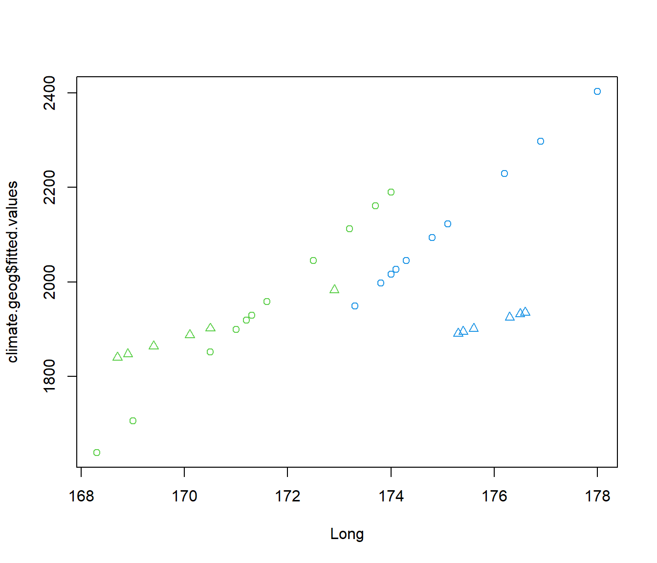 In the plot, green locations are for the South Island and blue for the North Island, triangles represent inland places and circles are places by the sea. The plot indicates, that, for coastal towns/cities, locations on the eastern side of each island (higher longitude) tend to have more sun than locations on the western side. But for inland places the slope is small - the effect of longitude it very little.
If we wanted to, we could try entering the other weather variables. We will stop here.