Lecture 17 Linear Models with Factors
So far we have focused on regression models, where a continuous random response variable is modelled as a function of one or more numerical explanatory variables.
Another common situation is where the explanatory variables are categorical variables, or factors.
In this lecture we will begin to look at such models, and will focus in particular on one-way models.
17.1 The One-Way Model
The one-way (or one factor) model is used when a continuous numerical response Y is dependent on a single factor (categorical explanatory variable).
In such models, the categories defined by a factor are called the levels of the factor.
17.2 Stimulating Effects of Caffeine
Question: does caffeine stimulation affect the rate at which individuals can tap their fingers?
Thirty male students randomly allocated to three treatment groups of 10 students each. Groups treated as follows:
Group 1: zero caffeine dose
Group 2: low caffeine dose
Group 3: high caffeine dose
Allocation to treatment groups was blind (subjects did not know their caffeine dosage).
Two hours after treatment, each subject tapped fingers as quickly as possible for a minute. Number of taps recorded.
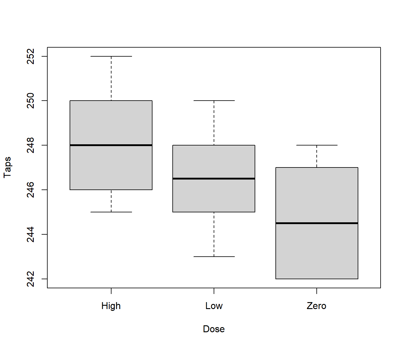
Number of taps is the response variable, caffeine dose is the explanatory variable. Here caffeine dose is a factor with 3 levels - zero, low and high. Does the apparent trend in the following boxplot provide convincing evidence that caffeine affects tapping rate?
17.3 Mathematical Formulation of the One-Way Model
The one-way model can be written as \[Y_{ij} = \mu + \alpha_i + \varepsilon_{ij}~~~~~~~~(i=1,\ldots,K,~~~~~j=1,\ldots,n_i)\]
where:
\(Y_{ij}\) is the response of the \(j\)th unit (observation) at the \(i\)th level of the factor;
\(K\) denotes the number of levels of the explanatory factor;
\(n_i\) is the number of observations (replications) at level \(i\) of the factor;
the values \(\varepsilon_{11}, \ldots,\varepsilon_{Kn_K}\) are random errors satisfying assumptions A1 to A4.
The mean response is \[E[Y_{ij}] = \mu + \alpha_i\]
17.4 Parameterisation of the One-Way Model
As it currently stands, the model defined by \[Y_{ij} = \mu + \alpha_i + \varepsilon_{ij}~~~~~~~~(i=1,\ldots,K,~~~~~j=1,\ldots,n_i)\] is overparameterised.
This means that there are multiple choices of values for the parameters that produce a model with exactly the same mean responses.
Suppose the factor has \(K = 2\) levels. Then \[E[Y_{1j}] = \mu + \alpha_1~~~~~~~~~~\mbox{and}~~~~~~~~~~~E[Y_{2j}] = \mu + \alpha_2\] Both of the following sets of parameter values give identical mean responses at both levels:
\(\mu = 10\), \(\alpha_1 = 4\), \(\alpha_2 = 8\).
\(\mu = 14\), \(\alpha_1 = 0\), \(\alpha_2 = 4\).
17.5 Solution to Overparameterisation
We impose a constraint on the parameters \(\alpha_1, \alpha_2, \ldots, \alpha_K\).
The two most popular (and easily interpretable) constraints are:
Sum constraint: \(\sum_{i=1}^K \alpha_i = 0\). In this case \(\mu\) can be interpreted as a kind of “grand mean”, and \(\alpha_1, \alpha_2, \ldots, \alpha_K\) measure deviations from this grand mean.
Treatment constraint: \(\alpha_1 = 0\). In this case level 1 of the factor is regarded as the baseline or reference level, and \(\alpha_2, \alpha_3 \ldots, \alpha_K\) measure deviations from this baseline. This is highly appropriate if level 1 corresponds to a control group, for example.
We will work with the treatment constraint. It is also used by default for factors in R.
17.6 Expressing Factorial Models as Regression Models
We can express a one-way factorial model as a regression model by using dummy (indicator) variables.
Define dummy variables \(z_{11}, z_{12}, \ldots, z_{n K}\) by \[z_{ij} = \left \{ \begin{array}{ll} 1 & \mbox{unit *i* observed at factor level *j*}\\ 0 & \mbox{otherwise.} \end{array} \right .\]
17.7 Regression form of one-way factor model
A one-way factor model can be expressed as follows: \[Y_i = \mu + \alpha_1 z_{i1} + \alpha_2 z_{i2} + \ldots + \alpha_K z_{iK} + \varepsilon_i~~~~~(i=1,2,\ldots,n)\]
This has the form of a multiple linear regression model. The dummy variables are binary predictors, which we covered in the previous lecture.
The parameter \(\mu\) is the regression intercept and, under the treatment constraint (\(\alpha_1 = 0\)), corresponds to the mean baseline (factor level 1) response.
17.8 Modelling the Caffeine Data
Our one-way factor model, where the factor has three levels, can be expressed as follows: \[Y_i = \mu + \alpha_2 z_{i2} + \alpha_{3} z_{i3} + \varepsilon_i\]
where:
\(Y_i\) is the number of taps recorded for the \(i\)th subject
\(z_{i2} = 1\) if subject \(i\) is on low dose; \(z_{i2} = 0\) otherwise;
\(z_{i3} = 1\) if subject \(i\) is on high dose; \(z_{i32} = 0\) otherwise.
Then, \(\mu\) is mean response for a subject on zero dose; \(\alpha_2\) is the effect of low dose in contrast to zero dose; and, \(\alpha_3\) is the effect of high dose in contrast to zero dose.
We will see that, rather than creating by hand the indicator variables, the factor() function in R does that automatically.
17.9 Expressing Factorial Models using Matrices
Since factorial models can be expressed as linear regression models, they may be described using matrix notation as we saw earlier.
For a one-way factorial model with treatment constraint: \[{\boldsymbol{y}} = X {\boldsymbol{\beta}} + \varepsilon\] where: \[{\boldsymbol{y}} = \left [ \begin{array}{c} Y_1\\ Y_2\\ \vdots\\ Y_n \end{array} \right ] ~~~~X = \left [ \begin{array}{cccc} 1 & z_{12} & \ldots & z_{1K}\\ 1 & z_{22} & \ldots & z_{2K}\\ \vdots & \vdots & \ddots & \vdots\\ 1 & z_{n2} & \ldots & z_{nK} \end{array} \right ] ~~~ {\boldsymbol{\beta}} = \left [ \begin{array}{c} \mu\\ \alpha_2\\ \vdots\\ \alpha_K\\ \end{array} \right ] ~~~ \boldsymbol{\varepsilon} = \left [ \begin{array}{c} \varepsilon_1\\ \varepsilon_2\\ \vdots\\ \varepsilon_n\\ \end{array} \right ]\]
There is no \(\alpha_1\) in the parameter vector, and no row for \(z_{i1}\) in the design matrix, because of the treatment constraint.
17.10 Design Matrix for Modelling the Caffeine Data
Write down the one-way model for the caffeine data using matrix notation. Take care to properly specify the design matrix.
17.11 Factorial Models as Regression Models
Since factorial models can be regarded as regression models, all ideas about parameter estimation, fitted values etc. follow in the natural manner.
Parameter estimation can be done by the method of least squares, to give vector of estimates \(\hat {\boldsymbol{\beta}} = (\hat \mu, \hat \alpha_2, \ldots, \hat \alpha_K)^T\).
Fitted values and residuals are defined in the usual way.
17.12 Back to the Caffeine Data
17.12.1 R Code
The factor levels of Dose have a natural ordering. In particular, it is intuitive to set the zero level as baseline (factor level 1).
## Caffeine <- read.csv(file = "caffeine.csv", header = T)
str(Caffeine)
'data.frame': 30 obs. of 2 variables:
$ Taps: int 242 245 244 248 247 248 242 244 246 242 ...
$ Dose: chr "Zero" "Zero" "Zero" "Zero" ...head(Caffeine) Taps Dose
1 242 Zero
2 245 Zero
3 244 Zero
4 248 Zero
5 247 Zero
6 248 Zerolevels(Caffeine$Dose)NULLCaffeine$Dose <- factor(Caffeine$Dose, levels = c("Zero", "Low", "High"))
levels(Caffeine$Dose)[1] "Zero" "Low" "High"The factor() command transforms the Dose variable from a character (i.e text) variable into a categorical variable (a factor) with levels. Specifying the levels with the levels argument reorders
the factor levels so that zero, low and high dose are interpreted as
levels 1, 2 and 3 respectively. Note that if we do not specify the order of the levels in the
factor() function, alphabetical order will be used (so in this case High would be the first level).
Fitting the Model Can use lm() function in R to fit model
in the same manner as for regression models.
Caffeine.lm <- lm(Taps ~ Dose, data = Caffeine)
summary(Caffeine.lm)
Call:
lm(formula = Taps ~ Dose, data = Caffeine)

Residuals:
   Min     1Q Median     3Q    Max
-3.400 -2.075 -0.300  1.675  3.700

Coefficients:
            Estimate Std. Error t value Pr(>|t|)
(Intercept) 244.8000     0.7047 347.359  < 2e-16 ***
DoseLow       1.6000     0.9967   1.605  0.12005
DoseHigh      3.5000     0.9967   3.512  0.00158 **
---
Signif. codes:  0 '***' 0.001 '**' 0.01 '*' 0.05 '.' 0.1 ' ' 1

Residual standard error: 2.229 on 27 degrees of freedom
Multiple R-squared:  0.3141,    Adjusted R-squared:  0.2633
F-statistic: 6.181 on 2 and 27 DF,  p-value: 0.006163
17.12.2 Final Comments
Recall, we have 30 male students randomly allocated to 3 treatment groups of 10 students each.
Groups treated with zero, low and high caffeine doses respectively.
Response variable is number of finger taps in a minute, explanatory variable is caffeine dose.
Using the notation introduced earlier, the parameter estimates are \(\hat \mu = 244.8\), \(\hat \alpha_2 = 1.6\) and \(\hat \alpha_3 = 3.5\).
The fitted values are:
| Dose (level) | mean response | fitted value |
|---|---|---|
| Zero (1) | \(\mu\) | 244.8 |
| Low (2) | \(\mu + \alpha_2\) | 246.4 |
| High (3) | \(\mu + \alpha_3\) | 248.3 |