Lecture 18 Interpretation of One-Way Models
In this lecture, we will consider hypothesis tests for one-way models.
We also look at model diagnostics for these models.
18.1 Similarities in Analysis for Factorial and Regression Models
Factorial models (using the treatment constraint) can be written as multiple linear regression models, using dummy variables:
\[Y_i = \mu + \alpha_2 z_{i2} + \ldots + \alpha_K z_{iK} + \varepsilon_i \quad(i=1,2,\ldots,n)\]
Why is there no \(\alpha_1 z_{i1}\)?
18.2 Differences in Analysis for Factorial and Regression Models
Despite the two models being similar in how they are expressed, there are differences in the way these types of model should be analysed.
Importantly:
- In a multiple linear regression model it makes sense to add or remove a single explanatory variable.
- In a factorial model it (usually) only makes sense to add or remove a whole factor, not single levels of a factor.
- This will usually require F tests (not just t-tests for single parameters).
18.3 Testing for Factor Effect
Typically the primary question of interest for a one-way model is this: is the mean response dependent on the factor?
In the factorial model (with treatment constraint) this question is addressed by testing H0: \[\alpha_2 = \alpha_3 = \cdots = \alpha_K = 0\] versus H1: \[\alpha_2, \alpha_3, \ldots, \alpha_K~\mbox{not all zero}\]
Because this is a test involving multiple parameters we will usually need to perform an F test.
18.3.1 F tests for Factor Effect
Testing for the significance of the factor in a one-way model is the same as comparing the (nested) models: \[M0: Y_i = \mu + \varepsilon_i \quad (i=1,2,\ldots,n)\] and \[M1: Y_i = \mu + \alpha_2 z_{i2} + \ldots + \alpha_K z_{iK} + \varepsilon_i \quad (i=1,2,\ldots,n)\]
Retaining H0 corresponds to \(M0\) being adequate.
Accepting H1 corresponds to \(M1\) being better.
We can use the F tests for nested models developed earlier (since factorial models can be regarded as regression models).
The F test statistic is \[F = \frac{[RSS_{M0} - RSS_{M1}]/(K-1)}{RSS_{M1}/(n-K)}\]
Note that the model M1 contains K ‘regression’ parameters, namely \(\mu\) and \(\alpha_2, \alpha_3, \ldots, \alpha_K\) (assuming the treatment constraint).
If fobs is the observed value of the test statistic, and X is a random variable from an FK-1,n-K distribution, then the p-value is given by \(P= P(X \ge f_{\mbox{obs}})\)
18.3.2 Omnibus F Test for the Caffeine Data
You can Download caffeine.csv to replicate the following example.
## Caffeine <- read.csv(file = "caffeine.csv", header = TRUE)
Caffeine$Dose <- factor(Caffeine$Dose, levels = c("Zero", "Low", "High"))
Caffeine.lm <- lm(Taps ~ Dose, data = Caffeine)
summary(Caffeine.lm)
Call:
lm(formula = Taps ~ Dose, data = Caffeine)

Residuals:
   Min     1Q Median     3Q    Max
-3.400 -2.075 -0.300  1.675  3.700

Coefficients:
            Estimate Std. Error t value Pr(>|t|)
(Intercept) 244.8000     0.7047 347.359  < 2e-16 ***
DoseLow       1.6000     0.9967   1.605  0.12005
DoseHigh      3.5000     0.9967   3.512  0.00158 **
---
Signif. codes:  0 '***' 0.001 '**' 0.01 '*' 0.05 '.' 0.1 ' ' 1

Residual standard error: 2.229 on 27 degrees of freedom
Multiple R-squared:  0.3141,    Adjusted R-squared:  0.2633
F-statistic: 6.181 on 2 and 27 DF,  p-value: 0.006163
18.3.3 Alternative Test for the Effect of Caffeine
In general, you conduct a test for factor effects using the anova()
command.
For a one-way model, R returns the omnibus F test statistic and related quantities.
anova(Caffeine.lm)Analysis of Variance Table
Response: Taps
Df Sum Sq Mean Sq F value Pr(>F)
Dose 2 61.4 30.7000 6.1812 0.006163 **
Residuals 27 134.1 4.9667
---
Signif. codes: 0 '***' 0.001 '**' 0.01 '*' 0.05 '.' 0.1 ' ' 118.3.3.1 Conclusions from the ANOVA table
The observed F-statistic for testing for the significance of caffeine dose is f = 6.181 on K-1 = 2 and n-K = 27 degrees of freedom.
The corresponding P-value is P=0.0062; we therefore have very strong evidence against H0; i.e. finger tapping speed does seem to be related to caffeine dose.
The table of coefficients in the R output shows that the mean response difference between the high dose and control groups is a little more than twice as big as the difference between low dose and control group.
18.3.4 Interpretation of the ANOVA Table
Use the ANOVA table produced by R to answer the following questions on the caffeine data.
What is the residual sum of squares for the full model M1?
What is the mean sum of squares for the model M1?
What is the residual sum of squares for the null model M0, given below? \[M0: Y_i = \mu + \varepsilon_i~~~~~~~(i=1,2,\ldots,30)\]
What is the mean sum of squares for the model M0?
18.3.5 Diagnostics for Caffeine Data
We have tested whether the speed of students’ finger tapping is related to the caffeine dose received. As usual, the validity of our conclusions is contingent on the adequacy of the fitted model. We should therefore inspect standard model diagnostics.
par(mfrow = c(2, 2))
plot(Caffeine.lm)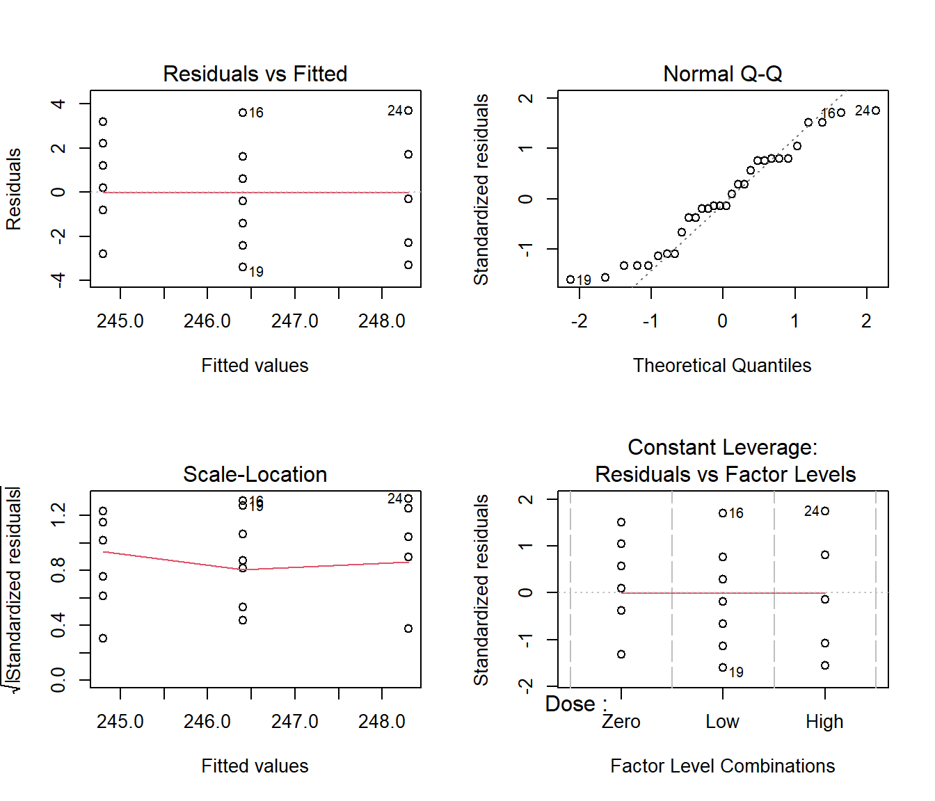
18.3.7 Comments on the Diagnostics: Application to the Caffeine Data
For factorial models, it is particularly important to scrutinize the plots for heteroscedasticity (non-constant variance), when the error variance changes markedly between the factor levels.
When heteroscedasticity is present, assumption A3 fails and conclusions based on F tests become unreliable.
The diagnostic plots do not provide any reason to doubt the appropriateness of the fitted model.
18.4 Bartlett’s Test for Heteroscedasticity
In order to assess heteroscedasticity, we can use the Bartlett’s test (or the Levene test).
The hypotheses for both tests are:
H0: error variance constant across groups versus
H1: error variance not constant across groups
Rejecting the null means that the equal variance assumption is violated.
18.4.1 Heteroscedasticity in Caffeine Data
Caffeine.bt = bartlett.test(Taps ~ Dose, data = Caffeine)
Caffeine.bt
    Bartlett test of homogeneity of variances

data:  Taps by Dose
Bartlett's K-squared = 0.18767, df = 2, p-value = 0.9104
The p-value for the Bartlett’s test is P=0.9104 which confirms that, for the caffeine data, we have no reason to doubt the constant variance assumption.
Caffeine.lt = leveneTest(Taps ~ Dose, data = Caffeine)
Caffeine.lt
Levene's Test for Homogeneity of Variance (center = median)
Df F value Pr(>F)
group 2 0.2819 0.7565
27 We reach the same conclusion with the Levene test.
18.3.6 Comments on the Diagnostic Plots: Technical
For a factorial model, the fitted values are constant within each group. This explains the vertical lines in the left-hand plots.
A balanced factorial design exists when the same number of observations are taken at each factor level.
When the data are balanced the leverage is constant, so a plot of the leverage would be pointless.
As a result, R produces a plot of standardized residuals against factor levels for balanced factorial models in place of the usual residuals versus leverage plot.